Goal of this simulation is finding the radius of an electron in an homogeneous magnetic field and checking the result against analytic.
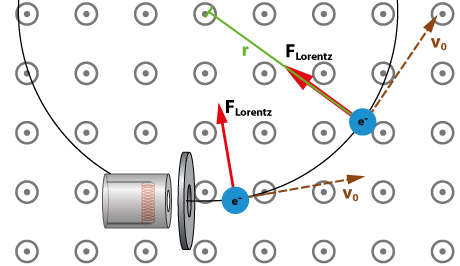
The Lorentz force is always perpendicular to the direction of motion of the electrons when electrons move in the B field. Further, it is the only acting force. Thus, the Lorentz force is the centripetal force necessary for a circular path. So it applies
\(\mathbf{F}_{Lorentz}=\mathbf{F}_{Zentripetal}\)
Inserting of \(\mathbf{F}_{Lorentz}=e \cdot v_{0} \cdot \mathbf{B}\) and \(\mathbf{F}_{Zentripetal}=m_{e} \frac{v_{0}^2}{r}\) leads to
\(e \cdot v_{0} \cdot \mathbf{B}=m_{e} \frac{v_{0}^2}{r}\)
Solving for r yields the formula for the radius of the circular path:
\(r=\frac{m_{e} \cdot v_{0}^2}{e \cdot \mathbf{B}}\)
This radius is also called ’Larmor Radius’.
Reference:
www.didaktik.physik.uni-muenchen.de/elektronenbahnen/b-feld/B-Feld/Auswertung.php
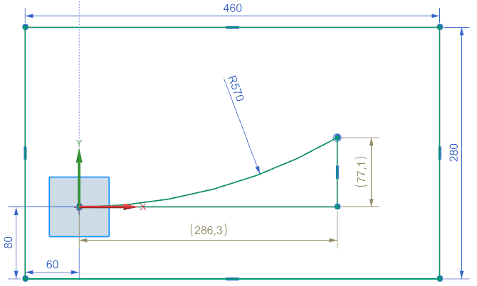
The picture below shows a sketch of the simulation model. The model
we use to simulate for the electron deviation uses following
properties.
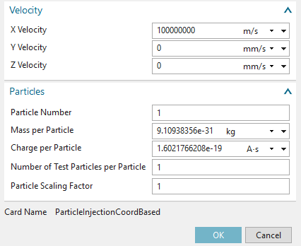
B = 0.001 T
me = 9.109e-31 Kg
\(V_{0} = 1e8\) m/s
e = 1.602e-19 C
Analytic radius result: r=570 mm
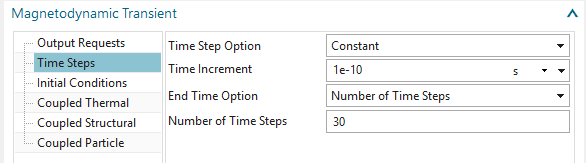
Time Step: 1e-10 s
Number of Time Steps: 30
Expected total displacement: 300 mm
Expected x,y displacement (from sketch): 286.3 mm, 77.1 mm
All particles start from the coordinate center in x direction. A circle with radius 570 mm and arc length 300 mm shows the way particles should go as expected from the analytic result. With an element size of 5 mm the electrons will jump over two element with each time step.
The simulation result is as follows.
Total displacement: 297.2 mm (deviation 0.9%)
x displacement: 286.8 mm (deviation 0.17%)
y displacement: 77.74 mm (deviation 0.82%)
Small deviations occur between simulation and analytics. These can come from the bidirection effect that is not included in the analytic formula. This may also come from the quite large jump at each time step.
Necessary time: 20 min. The model is already build and ready to solve. To perform this simulation follow these steps:
Download the model files for this tutorial from the following
link:
https://www.magnetics.de/downloads/Tutorials/11.CouplParticle/11.2LarmorRadius.zip
Start the Program Simcenter ![]() (or
NX). Use Version 12 or higher.
(or
NX). Use Version 12 or higher.
In Simcenter, open ![]() the file
’LarmorRadiusCheck_sim1.sim’.
the file
’LarmorRadiusCheck_sim1.sim’.
Edit the solution ’MagDynPicBi’ and check register ’Time
Steps’.
check register ’Coupled Particle’.
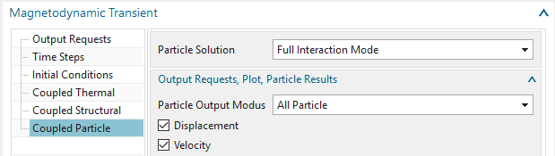
Check the simulation object ’Particle Injection(1)’
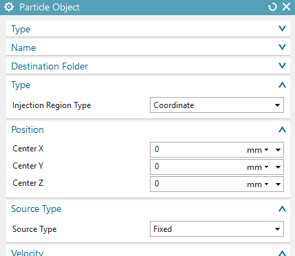
Solve the solution: Click on ![]() and OK. The solver will run about 3 min.
and OK. The solver will run about 3 min.
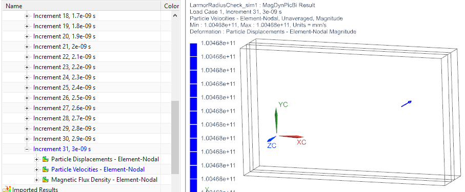
after the solve has finished open the ’Particle Displacement’ result.
set the time step to the last and read the result for x and y displacement. These values should be as discussed above.
check for other results as desired. Following picture shows the
velocity at the last step.
This tutorial is complete.