Tutorial 1

Particle Accelerator Pipe

The following three examples are intended to show the principal functionalities of the Particle Solver in the context of a linear particle accelerator. In particular the flexibility of the Solver will be demonstrated, in the context of a Magentodynamic, a Magnetistatic and an Electrostatic simulation. The three examples are based on each other, and should thus be executed in consecutively.

Bunched Particles – Magnetodynamic

Abstract: A bunch of particles starts with a velocity of 15 \(\tfrac{\mathrm{mm}}{\mathrm{s}}\) from the displayed particle source and is headed towards an accelerator pipe with a constant electric field of 1 \(\tfrac{\mathrm{V}}{\mathrm{mm}}\), in order to be linearly accelerated. Both the displacements and the velocities will be evaluated and compared to calculated values.

Estimated time: 0.5 h

Follow the steps:

1. Download the model files for this tutorial from the following link:
   https://www.magnetics.de/downloads/Tutorials/11.CouplParticle/11.1ParticlePipe.zip

2. Open the file ’ParticlePipe.prt’.

3. Observe the dimensions of the particle source (red), the accelerator pipe (green) and the air (blue).

   • The particle source is a cube comprising 15 \(\mathrm{mm}\) edges;

   • The accelerator is a cylinder of length 100 \(\mathrm{mm}\) (and radius 15 \(\mathrm{mm}\));

   • The accelerator rear face is distanced 150 \(\mathrm{mm}\) from the origin; and 142.5 \(\mathrm{mm}\) from the front face of the source;

   • The accelerator front face is distanced 375 \(\mathrm{mm}\) from the front boundary of the surrounding air box.

   \(\Rightarrow\) In summary the three vital distances are 100 \(\mathrm{mm}\), 150 \(\mathrm{mm}\) and 375 \(\mathrm{mm}\).

4. Switch to Simcenter Pre/Post

5. Create a new FEM and Simulation. Choose Solver MAGNETICS and Analysis Type ’3D Electromagnetics’. Switch off the ’Create idealized Part’.

   

6. Choose Solution Type ’Magnetodynamic Transient’.

   • In register ’Output Requests’ under ’Plot’ activate ’Magnetic Fluxdensity’ to enable the calculation of the B field. Moreover, the Magnetic Potential (a-Pot) and ’Electric Fieldstrength’ might be interesting (but not vital) for this tutorial.

     

   • Under ’Time Steps’ select a ’Time Increment’ of 1 \(\mathrm{s}\); and under ’Number of Time Steps’ a total of 50 time steps.

     

   • In register ’Coupled Particle’ set the ’Particle Solution’ to ’Full Interaction Mode’. With this selection the Particle Solver is bi-directionally coupled with the field solver, meaning that the EM fields accelerate/deflect the particles; and in turn the particles modify the sources and currents for the field solver (for more information THEORY). Also set the ’Particle Output Mode’ to ’All Particle’ and select ’Displacements’, ’Velocity’ and ’Mass’ as Output.

     

   • In register ’Initial Conditions’ accept the default magnetic condition ’Zero Vector Potential’.

   • Press ’Ok’.

7. Next, switch to the FEM environment and make it a ’Displayed Part’ (right click on the “.fem” file)

   • First, create ’Mesh Matings’ for all three bodies; resulting in 9 MMC.

     

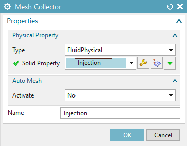
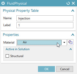
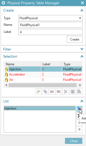
   • Then, create a new Collector (right click on ’3D Collectors’; and then ’New Collector’). Call This Collector Injection; and assign a Type ’Fluid Physical’. Create a new Physical called Injection and assign ’Air’ as Material

     

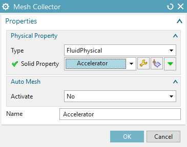
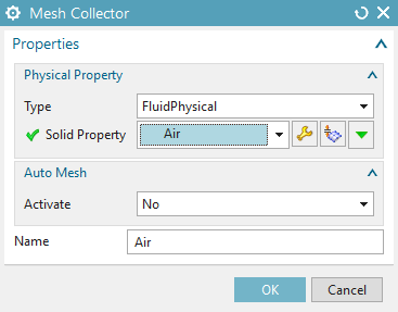
     Repeat this process two more times, i.e. create a new Collector called Accelerator and one called Air (also assign Type ’Fluid Physical’ and Material ’Air’)

     

   • Mesh the injection source with a ’3D Swept Mesh’ of size 6mm; herein set the option ’Attempt Quad Only’ to ’On-Zero Triangles’. The meshing should result in a regular hex-mesh with a total of 27 Cells.

     

   • Mesh the accelerator pipe with a ’3D Tetrahedral’ mesh of size 9.1mm; or a finer mesh.

     

   • Mesh the surrounding air volume with a ’3D Tetrahedral’ mesh of size 44.9mm; or a finer mesh.

     

   • In the top slider select ’Magnetics’ and click ’Rename Meshes By Collectors’; then switch back to ’Home’.

8. Next, switch to the SIM environment (right click on the “.fem” file; then click ’Display Simulation’)

   • In the SIM environment, create create a \(A=0\) boundary condition. To do so right click on ’Constraints’ and select ’Flux tangent’; then select the six faces of the air volume.

     

   • Now, create an particle source. To do so right click on ’Simulation Objects’, then ’New Simulation Object’; and select ’Particle Object’

     

     
     Then, specify the type to be ’Particle Source, Mesh-Based’ and set the ’Injection Region Type’ to ’Volume’.
     
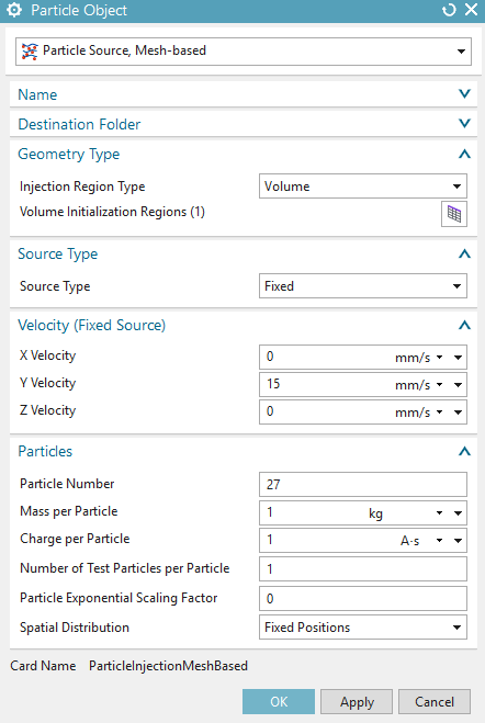
     Note.: The above source provides a total of 27 particles (1 Testparticle) with Mass 1 \(\mathrm{Kg}\) and Charge 1 \(\mathrm{A \cdot s}\) that travel with an initial velocity of 15 \(\tfrac{\mathrm{mm}}{\mathrm{s}}\) in Y-direction.
     
     Last, create the Volume Initialization Region. Thus, click on ’Create Volume Intialization Regions’. Then, select the Injection Physical and add it to the list. Press ’Ok’.

   • Finally, create an accelerator pipe. Again right click on ’Simulation Objects’ and ’New Simulation Object’; but now select ’Acceleration and Deflection Pipe’. Select the type to be ’Acceleration’ and assign an Electric Y field of 0.002 (this provides an \(E_y\) field of 0.002 \(\tfrac{\mathrm{V}}{\mathrm{m}}\)).

     

     
     Note.: The Acceleration and Deflection Pipes are provided to create constant electric and/or magnetic fields which can be used to accelerate and/or deflect particles. In the selected areas these fields are held constant (even despite other calculations that might be additionally created). Moreover, said fields are only visible for the particle solver. In a nutshell the pipes erase any field values in the specific regions and replace it with specified values for the Particle Solver.

   • Press ’Solve’ to solve the solution.

9. Switch to the Postprocessing environment (under “Results” double-click ’Magnetic’)

   • In the following the displacements and the velocities of the particles will be evaluated. Thus, let us first specify the required theory and adjust it to this example. The (mechanical) motion of the particles isdescribed by Newton’s second Law \[\begin{aligned} \mathbf{F} = \mathrm{m} \, \mathbf{a} = \mathrm{m} \, \mathbf{\ddot{x}}, \end{aligned}\] whereas the electromagnetic impact on the particles is given by the Lorentz Force / (assuming \(\mathbf{B}=0\), thus being the Coulomb Force) \[\begin{aligned} \mathbf{F}_L = \mathrm{q} \, \mathbf{E}. \end{aligned}\] Here, \(\mathrm{m}\) is the Mass, \(\mathrm{q}\) the charge and \(\mathbf{a}\) the acceleration. By simple integration we obtain \[\begin{aligned} \mathbf{a} (t) &= \tfrac{\mathrm{q}}{\mathrm{m}} \mathbf{E},\\ \mathbf{v} (t) &= \tfrac{\mathrm{q}}{\mathrm{m}} \mathbf{E} t + \mathbf{v}_0,\\ \mathbf{x} (t) &= \tfrac{1}{2} \tfrac{\mathrm{q}}{\mathrm{m}} \mathbf{E} t^2 + \mathbf{v}_0 t + \mathbf{x}_0. \end{aligned}\] As a consequence we deduce that an acceleration is only possible within the acceleration tube. In the field free Domains, Newtons first law applies on the particles: each particle moves with a constant velocity.

   • Let us set appropriate plot options: for the displacements we choose spheres (click on ’Edit Post View’. Under ’Display’ select ’Spheres’. Change the scale to 5.0 ’mm’), and arrows for the velocities (click on ’Edit Post View’. Under ’Display’ select ’Arrows’)

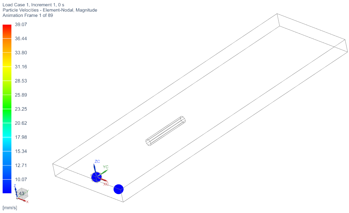
   • First, obeserve the overall particle motion. Thus, select ’Particle Velocities’, click ’Animate’; and under ’Animate’ select ’Iterations’. In total five timesteps (given by the Increments) are significant:

     Increment 1:

     at time \(t=0 \,\mathrm{sec}\) the particles are initialized in the source

     Increment 2:

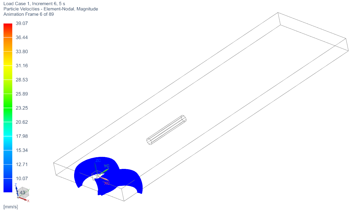
     at time \(t=1 \,\mathrm{sec}\) the first particles exit the source

     Increment 12:

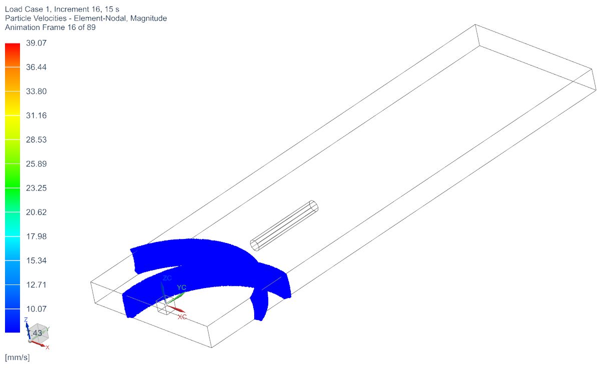
     at time \(t=11 \,\mathrm{sec}\) the first particles inpinge the accelerator

     Increment 16:

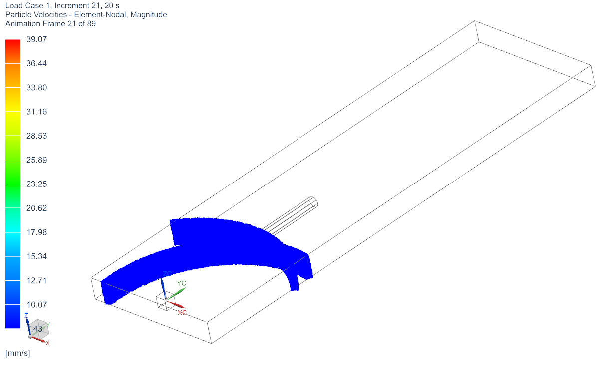
     at time \(t=15 \,\mathrm{sec}\) the first particles exit the accelerator

     Increment 31:

     at time \(t=30 \,\mathrm{sec}\) the last particles leave the air volume

     Let us now investigate these five incidents in detail.

   • At \(t=0 \, \mathrm{sec}\) the particles are initialized in the source. Observe that the displacement plot does not show anything. This is because there are no displacements present. The Velocities are set to 15 \(\tfrac{\mathrm{mm}}{\mathrm{s}}\) as has been set.

     

     
     It can be observed that there are 27 Particles present that are all initialized in the respective middle of each Cell within the Particle Injection (Remember that we have set 27 cells before). Consequently, the particles start in three fronts (with respect to the y direction). The first row starts at \(y=5\), the second at \(y=0\) and the third at \(y=-5\).

   • At \(t=1 \, \mathrm{sec}\) the particles in the first row have exited source. Now the displacement of the particles are visible. We observe displacements of 15 \(\mathrm{mm}\) and Velocities of 15 \(\tfrac{\mathrm{mm}}{\mathrm{s}}\).

     

     
     The observed Displacements and Velocities are expected. Since there is no electric Field Present the velocity stays constant thus resulting in, \(x(t) = v_0 \, \mathrm{t} = 15 \tfrac{\mathrm{mm}}{\mathrm{s}} \cdot 1 \mathrm{s} = 15 \mathrm{mm}\).
     Since we have chosen the distance between the particle source and the accelerator pipe to be 150 \(\mathrm{mm}\), we expect that the particles will travel 10 \(\mathrm{sec}\) to the accelerator pipe. Thus the first row particles should have entered the accelerator pipe after 11 \(\mathrm{sec}\), i.e. at Increment 12.

   • At \(t=11 \, \mathrm{sec}\) the particles in the first row have entered the accelerator pipe. We observe that the (max) velocity has changed to 17 \(\tfrac{\mathrm{mm}}{\mathrm{s}}\). Moreover the (max) displacement is now 167 \(\mathrm{mm}\).

     

     
     The observed Displacements and Velocities are again expected. Inside the accelerator pipe there is an electric field of 2 \(\tfrac{\mathrm{V}}{\mathrm{mm}}\) present. Thus we obtain an acceleration of \(a(t) = 1 \mathrm{A} \mathrm{s} \cdot \tfrac{1}{\mathrm{Kg}}\cdot 2 \tfrac{\mathrm{V}}{\mathrm{mm}}=2 \tfrac{\mathrm{mm}}{\mathrm{s}^2}\). With the starting velocity of 15 \(\tfrac{\mathrm{mm}}{\mathrm{s}}\) this results in a velocity of 17 \(\tfrac{\mathrm{mm}}{\mathrm{s}}\) after 1 \(\mathrm{sec}\) in the acceleration pipe. Therefore, also the displacements are expected: the particles have traveled 150 \(\mathrm{mm}\) to the pipe; here the velocity has changed to 17 \(\tfrac{\mathrm{mm}}{\mathrm{s}}\). Thus, after one timestep the particles are at 167 \(\mathrm{mm}\).
     
     We have choosen the accelerator pipe to be 100 \(\mathrm{mm}\) long. With the above acceleration we can calculate the time that the particles need to travel through this pipe: \[\begin{aligned} 100 \mathrm{mm} = 1 \tfrac{\mathrm{mm}}{\mathrm{s}^2} \cdot t^2 + 15 \tfrac{\mathrm{mm}}{\mathrm{s}} \cdot t \quad \Rightarrow \quad t_+= - \tfrac{15}{2} \mathrm{s} + \sqrt{\tfrac{225+400}{4} \mathrm{s}^2} \nonumber = 5 \mathrm{s}. \end{aligned}\] During this time the velocity is expected to change by 10 \(\tfrac{\mathrm{mm}}{\mathrm{s}}\).

   • At \(t=15 \, \mathrm{sec}\) the particles in the first row left the accelerator pipe. We observe that the (max) velocity has changed to 25 \(\tfrac{\mathrm{mm}}{\mathrm{s}}\). Moreover the (max) displacement is now 225 \(\mathrm{mm}\).

     

     
     The observed Displacements and Velocities are again expected. From the previous discussion we expect a velocity change of 10 \(\tfrac{\mathrm{mm}}{\mathrm{s}}\). With a starting velocity of 15 \(\tfrac{\mathrm{mm}}{\mathrm{s}}\) this results in a velocity of 25 \(\tfrac{\mathrm{mm}}{\mathrm{s}}\) after 15 \(\mathrm{sec}\). Therefore, also the displacements are expected: the particles have travelled 230 \(\mathrm{mm}\) to the end of the pipe while beeing accelerated; and one second with 25 \(\tfrac{\mathrm{mm}}{\mathrm{s}}\). Thus, this results in a total of 255 \(\mathrm{mm}\).
     
     In the remaining 375 \(\mathrm{mm}\) the particles should travel with a constant velocity of 25 \(\tfrac{\mathrm{mm}}{\mathrm{s}}\) for 15 \(\mathrm{sec}\).

   • At \(t=31 \, \mathrm{sec}\) the last particles have left the air volume. We observe that the velocity is 25 \(\tfrac{\mathrm{mm}}{\mathrm{s}}\). Moreover the (max) displacement is now 620 \(\mathrm{mm}\).

     

   • As a check we investigate the Magnetic Flux result; thus switch on the ’Magnetic Flux Density’ result.

     Remember that there is no external Magnetic Field Source (e.g. from a Coil or a Constraint etc.) in the simulation by default. The only source for a Magnetic field thus is by the particles. A moving particle \(i\) with velocity \(\mathbf{v}_i\) and charge \(q_i\) produces a Current \[\begin{aligned} \mathbf{J}_i = q_i \mathbf{v}_i, \end{aligned}\] whereas a total current \(\mathbf{J}\) is just the sum of all single particle currents, and can enter as a source into (Magnetodynamic) Amperes Law \[\begin{aligned} \nabla \times \mathbf{H} = \mathbf{J} = \underbrace{\mathbf{J}_s}_{=0} + \sum_i \mathbf{J}_i. \end{aligned}\]
     With this in mind, press ’Animate’ (remember to switch on the ’Iterations’ toogle); as a result we observe a (small) magnetic field in the wake of the particle bunch.
     
     Note.: The selected ’Full Interaction Mode’ allows the bi-directional coupling of sources and currents into Maxwells equations. In this example it thus enables to impose a current into Amperes Law.

Single Particle – Magnetostatic

Abstract: A single particle starts with a velocity of 15 \(\tfrac{\mathrm{mm}}{\mathrm{s}}\) from Coordinate \(\mathbf{x}_0 = (0,0,0)\) and heads towards an accelerator pipe with a constant electric field of 1 \(\tfrac{\mathrm{V}}{\mathrm{mm}}\), in order to be linearly accelerated. Here, a Magnetostatic solution with an uni-directional particle coupling is applied.

Estimated time: 0.1 h

Follow the steps:

1. In this example we directly start in the SIM environment. For the meshing we refer to steps 1-6 of the previous example.

2. In the solution bar press the ’Solution’ button; to create an additional solution.

   • As ’Solution Type’ select ’Magnetostatic’

   • In register ’Output Requests’ under ’Plot’ again activate ’Magnetic Fluxdensity’

   • Under ’Time Steps’ select a ’Time Increment’ of 1 \(\mathrm{s}\) with a total of 50 time steps

     

   • In register ’Coupled Particle’ set the ’Particle Solution’ to ’Dynamic Particle Mode’. With this selection the Particle Solver is uni-directionally coupled with the field solver, meaning that the EM fields accelerate/deflect the particles; but the particles do not impose any sources and currents. Also set the ’Particle Output Mode’ to ’All Particle’ and select ’Displacements’ and ’Velocity’ as Output.

     

   • Press ’Ok’.

3. Switch to the new Magnetostatic solution.

   • Within the new Magnetostatic solution, apply the previously used ’Flux Tangent’ BC; as well as the accelerator pipe (i.e. by dragging said objects into the solution from the respective containers)

   • Now, create a new ’Particle Source’ (i.e. right click on ’Simulation Objects’ and ’Particle Objects’)

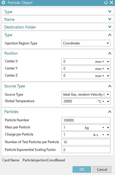
   • Then, specify the type to be ’Particle Source’ and set the ’Injection Region Type’ to ’Coordinate’.

     

     
     The above source provides one particle with Mass 1 \(\mathrm{Kg}\) and Charge 1 \(\mathrm{A \cdot s}\) that starts at position \(\mathbf{x}_0 = (0,0,0)\) and travels with an initial velocity of 15 \(\tfrac{\mathrm{mm}}{\mathrm{s}}\) in Y-direction.
     
     Note: In contrast to the previous mesh-based source, this source is coordinate based. Thus, the previous creation of a CAD geometry and subsequent meshing is not required for this type of source.

4. Press ’Solve’.

5. Switch to the ’Results’ environment.

   • The displacements and velocities of the particle behave similar as in the previous example. However, in this simplified scenario they are of course exact, meaning that there is no spread (we omit the calculation and refer to the previous example).

     

   • As a last check we investigate the Magnetic Flux result again; thus switch on the ’Magnetic Flux Density’ result. We observe that the Magnetic Flux Density is zero everywhere. This result is expected, since we have switched on the uni-directional coupling, meaning that the particles do not impose any sources or currents on the field solver, meaning \[\begin{aligned} \nabla \times \mathbf{H} = \mathbf{J} = \underbrace{\mathbf{J}_s}_{=0} = 0. \end{aligned}\]
     

Thermal Particle Initialization – Electrostatic

Abstract: Two particle sources are initialized with 1 Million particles, respectively. The particles are initialized with thermal velocities, i.e. each velocities absolute value corresponds to a particle in an ideal gas at \(20.000^\circ \mathrm{C}\); with directions choosen randomly. The sources are initiated at Coordinates \(\mathbf{x}_0^1 = (0,0,0)\) and \(\mathbf{x}_0^2 = (0,0,0)\) and an accelerator pipe with a constant electric field of 1 \(\tfrac{\mathrm{V}}{\mathrm{mm}}\) is employed. Here, an Electrostatic solution with an uni-directional particle coupling is applied.

Estimated time: 0.25 - 0.5 h (hardware dependent)

Follow the steps:

1. In this example we directly start in the SIM environment, again. For the meshing we refer to steps 1-6 of example 1.

2. In the solution bar press the ’Solution’ button; to create an additional solution.

   • As ’Solution Type’ select ’Electrostatic’

   • In register ’Output Requests’ under ’Plot’ we deselect all Output.

   • Under ’Time Steps’ select a ’Time Increment’ of 1 \(\mathrm{s}\) with a total of 100 time steps

     

   • In register ’Coupled Particle’ set the ’Particle Solution’ to ’Static Particle Mode’.

     

     
     With this selection the Particle Solver is uni-directionally coupled with the field solver, meaning that the EM fields accelerate/deflect the particles; but the particles do not impose any sources and currents. In addition the Fields are only passed to the particle solver at initial time, i.e. one time only. Also set the ’Particle Output Mode’ to ’All Particle’ and select ’Displacements’, ’Velocity’ and ’Type’ as Output.

   • Press ’Ok’.

3. Switch to the new Electrostatic solution.

   • In the SIM environment, apply the acceleration pipe from the previous examples (i.e. drag it into the ’Simulation Objects’).

   • Now, create a \(\varphi=0\) boundary condition. To do so right click on ’Constraints’ and select ’Given phi-Pot by Math-Function’; then select the six faces of the air volume.

     

   • Now, create two new ’Particle Sources’ (i.e. right click on ’Simulation Objects’ and ’Particle Objects’)

   • Then, specify the types to be ’Particle Source’ and set the ’Injection Region Type’ to ’Coordinate’, respectively (apply \(\mathbf{x}_0^1 = (0,0,0)\) and \(\mathbf{x}_0^2 = (0,75,-10)\)). Under ’Velocity Distribution’ select ’Full Thermal’ with a ’System Temperature’ of \(20.000^\circ \mathrm{C}\).

     

     
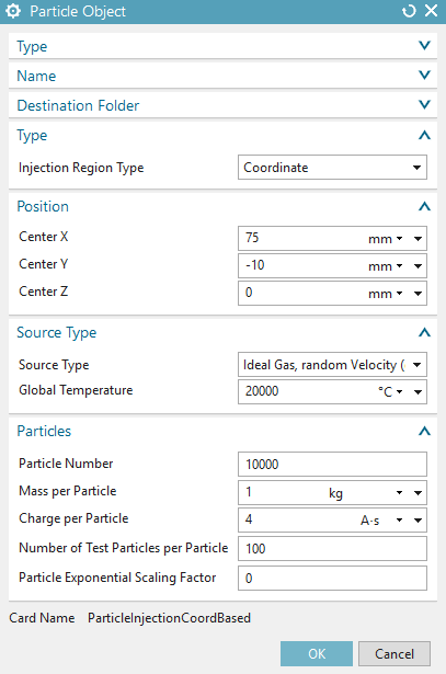
     The above sources provide one Million particles each, that are initialized with thermal distributions. In the first source 100.000 Particles with 10 Testparticles each are initialized with Mass 1 \(\mathrm{Kg}\) and Charge 1 \(\mathrm{A \cdot s}\), whereas in the second source 10.000 Particle with 100 Testparticles each are initialized with Mass 1 \(\mathrm{Kg}\) and Charge 4 \(\mathrm{A \cdot s}\).
     
     Note: Testparticles are used for statistic averaging (i.e. to obtain a certain Liouville average within a Plasma Simulation). Thus, the effect of Testparticles is similar to that of smearing.

4. Press ’Solve’ (the Solve will take some time).

5. Switch to the ’Results’ environment.

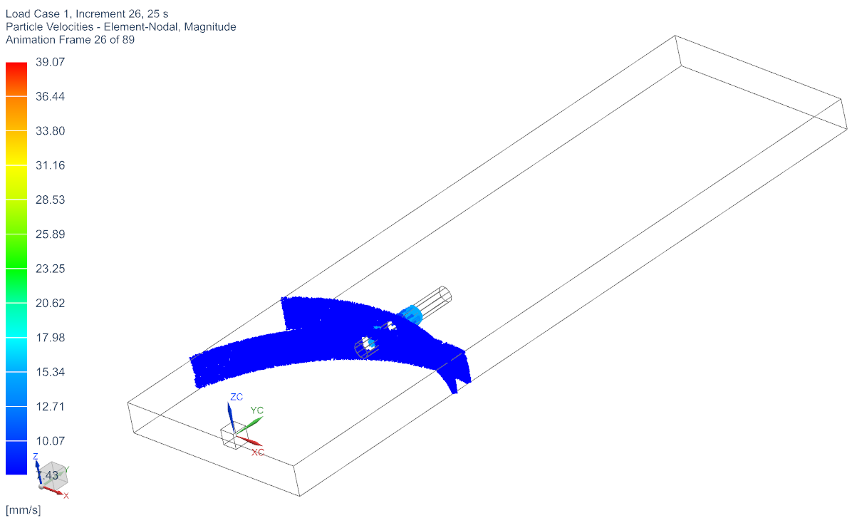
   • In the following we will solely investigate the particle velocities, thus click on the ’Particle Velocities’ result. To obtain a decent plot select ’Edit Post View’ and switch the ’Color Display’ to ’Arrows’. Then switch the ’Size’ to ’Result’ and select a suiting ’mm’ value, such as 10 \(\mathrm{mm}\).

   • Then start an Animation, i.e. press the ’Animate’ button ( and remember to switch on the ’Iterations’ toogle). The plotting process may take a while since many particles to be plot are present. When the Animation is finished, observe the particle evolution.

   • Due to the fact that very many particles are present, we observe a wave-like behaviour of non-interacting particles. In particular we see two “furball”-like structures at time \(t=0\, \mathrm{sec}\) around the two sources, from which wave-fronts are spherically expanding with ongoing time.

     
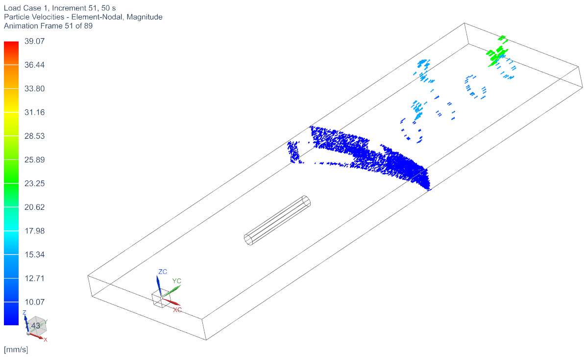
     Until 20 \(\mathrm{sec}\) the particles from the two sources move at the same abolute velocities (but with different directions). This is expected, since the velocities are just the starting velocities; and are not changed, due to the absence of any forces. Indeed this behaviour is the same as in the previous examples (just with more particles).

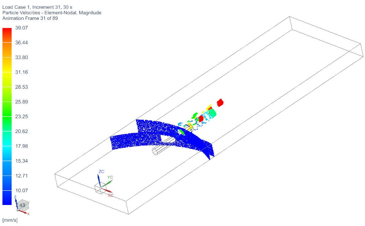
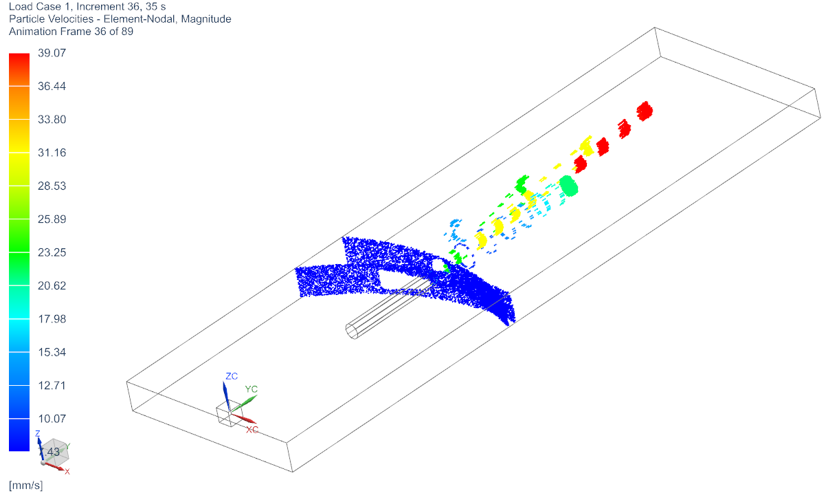
   • After (roughly) 20 \(\mathrm{sec}\) the first particles start impinging on the accelerator pipe, and are accelerated by the electric field (of 2 \(\tfrac{\mathrm{V}}{\mathrm{mm}}\) in Y-direction). After 30 \(\mathrm{sec}\) we obtain a difference in the change on the velocities of the particles from the two sources. The particles from the second source at \(\mathbf{x}_0^2\) are accelerated four times faster than the particles from the first \(\mathbf{x}_0^1\). Moreover, said particles are moving slightly to the left.

     
     Again the observed results are expected. Recall that the particles from the second source were initialized with four times larger charges 4 \(\mathrm{A\cdot s}\). Due to \(\mathbf{a} (t) = \tfrac{\mathrm{q}}{\mathrm{m}} \mathbf{E}\) they are thus accelerated four times faster. In addition the second particle source has been offset by 75 \(\mathrm{mm}\) right to the first particle source. As a result the particles are inpinging at the accelerator pipe under a larger angle and also exit the accelerator pipe under a larger angle.

The tutorial is complete