Electrostatic

Microstrip Line (Beginner)

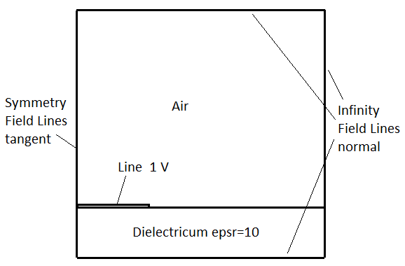
In this example it is shown how to analyze a simple 2D electrostatic problem. The geometry is a section of a microstrip line. It is symmetric, that’s why only one half of the section is modeled. The simulation is possible to set up in 2D or in 3D. Following we work in 2D but both 2D and 3D models are available in the tutorials folder.

Estimated time: 30 min
Follow these steps in Simcenter

Preparations

1. download the model files for this tutorial from the following link:
   https://www.magnetics.de/downloads/Tutorials/1.EleSta/1.1mStrip.zip

2. unzip the archive. There will be one folder ’start’ and one ’complete’.

3. Start the Program Simcenter (or NX). Use Version 10 or higher.

4. In Simcenter, click Open and navigate to folder ’start’. Select the file ’mStrip.prt’ and click OK. (Maybe you must set the file filter to ’prt’)

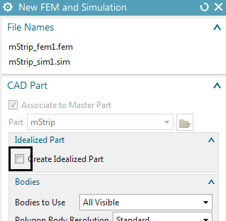
5. Create New FEM and Simulation

6. Swith off ’Create Idealized Part’ (picture below) because there is no need for doing simplifications.

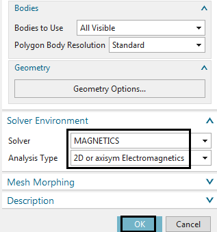
7. Choose Solver ’MAGNETICS’, Analysis Type ’2D or axisym Electromagnetics’ and click OK.
   

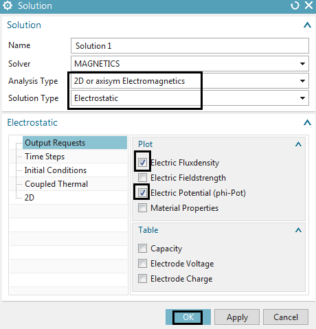
8. A new window opens to define the solution. Choose Solution Type ’Electrostatic’.

9. In tab ’Output Requests’ activate

   • ’Electric Fluxdensity’ and

   • ’Electric Potential (phi-Pot)’

   • Click OK to finish the solution definition.
     

Fem File Steps

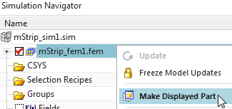
1. Set the Fem file to the displayed part.
   

2. Mesh the Dielectricum

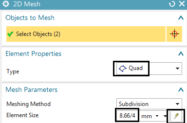
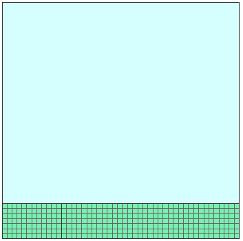
   • Click on ’2D Mesh’ and select the two bottom faces under the mStrip line (green in below picture).

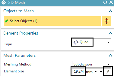
   • Set the Type to ’Quad’.
     Hint: Tri elements are also possible of course, but this geometry is perfect for Quads.

   • Click on ’Automatic Element Size’ to ask the system for a convenient element size. Divide this value by 4 to allow small elements in this area.
     

3. Assign Properties for the Dielectricum

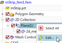
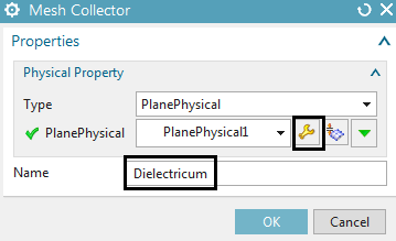
   • Double click the newly created mesh collector ’Plane(1)’. A new window appears. Accept the default type ’PlanePhysical’.

   • Change the Name to ’Dielectricum’.

   • To change the properties of this choose ’Edit’ (Picture below right)
     

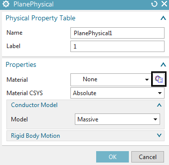
   • for assigning the material select the button ’Choose Material’ (Picture below left). A new window appears showing the Material List.

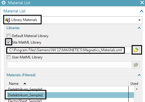
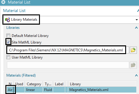
   • In the Material List activate ’Library Materials’ and ’Site MatML Library’.

   • Choose the browse function and insert the MAGNETICS material library from your installation directory. In a usual Simcenter or NX12 installation this will be something similar to this:
     ’.../NX 12.0/MAGNETICS/Magnetics_Materials.xml’

   • From the Material List select the material ’Dielektrikum_Sample2’
     

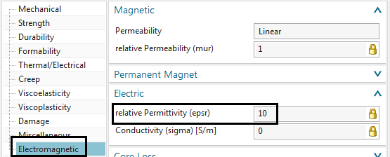
   • Hint: To check the properties of the selected material choose ’Inspect Material’ . In register ’Electromagnetic’ check for the correct setting of the relative Electric Permittivity (epsr):
     

   • Click Close, OK, OK, OK to finish the definition of dielectricum.

4. Mesh the air:

   • Click on ’2D Mesh’ and select the upper face.

   • Set the Type to ’Quad’ and click on ’Automatic Element Size’ to ask the system for a convenient element size. Divide this value by 4.
     

5. Assign Properties for Air

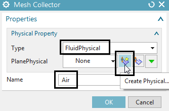
   • Edit the newly created mesh collector ’Plane(2)’. Change the Type to ’FluidPhysical’ and the Name to ’Air’.

   • Then click ’Create Physical’ to create a new physical property for air. In the following window click ’Choose material’
     

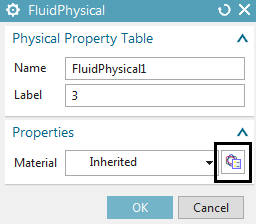
   • Select the material ’Air’ from the same library as before.
     

   • Click Close, OK, OK to finish the definition of air.

6. For easier post processing, click on the button ’Rename Meshes ...’ from the Magnetics toolbar. That utility renames all meshes and therefore is a useful feature especially with larger models and many meshes.

Sim File Steps

1. Switch to the Sim file
   

2. Hint: Possible Constraints in Electrostatics are

   • Given phi-Pot by Math-Function
     Use this function to assign a mathematical function or simply a value for Voltage

   • Perfect Conductivity Boundary
     This condition simulates the behavior of a perfect conductor e.g. there will be a constant voltage. The magnitude of this voltage will be calculated by MAGNETICS

3. Hint: Possible Loads are

   • Charge [A*s]

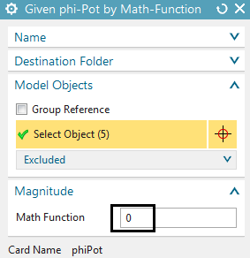
4. To create a constraint that results in normal field lines at the outside edges:

   • Click on ’Given phi-Pot by Math-Function’ and select the 5 outside edges, but not the symmetry edges (see picture below right).

   • Assign a Magnitude of 0. Click OK.
     

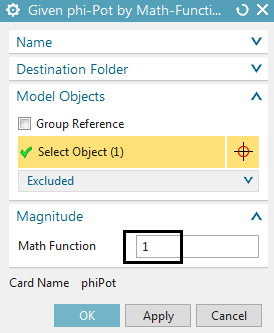
5. To assign the constraint ’1 V’ on the microstrip line (see picture below):

   • Click on ’Given phi-Pot by Math-Function’ and select the microstrip edge.

   • Assign a Magnitude of 1. Click OK.
     

6. Solve the Solution: Click on ’Solve’ and OK.

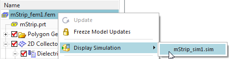
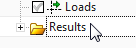
7. Perform Post Processing:

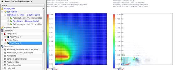
   • Double click the Result. The Simcenter system switches to the Post Processing Navigator.
     

   • In the Post Processing Navigator double click the Electric Potential Result or any other to see its field plot.

   • The picture below shows on the left side the electric potential and on the right side the electric flux density result with arrows.
     

8. The tutorial is complete. Save your files and close them.