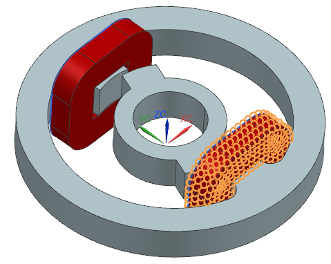
The problem 24 is for validating 3D nonlinear time transient codes. The user can read the document ’problem24_withResults.pdf’ to get further background information for this problem.
In this problem we switch on the Voltage in two coils to a value of
23.1 V. We calculate the time dependent current in the coils, the torque
and flux density over time.
Estimated time: 1.5 h
The task description does not give any information about the
conductivity of the coil material. Instead it provides the ohm
resistance: Both coils have 3.09 Ohm, so one will have the half of it.
To account for this given resistance in our simulation there are two
possibilities: We can either adjust the conductivity or the fill-factor
of the coil to drive the resistance to the demanded value.
So our strategy will be building up the model using standard copper and
first performing a fast static analysis to compute the ohm resistance of
the coils. This first solution will be done without rotor and stator,
just with the coils and air. Comparing this ohm value against the
demanded one will give us a scale value. This scale value can be used to
either scale the coil conductivity or the coil fill-factor. We will use
the fill-factor. After this the transient run can be done.
download the model files for this tutorial from the following
link:
https://www.magnetics.de/downloads/Tutorials/4.MagDyn/4.2Team24.zip
unzip the archive. There will be one folder ’start’ and one ’complete’.
Start the Program Simcenter ![]() (or
NX).
(or
NX).
In Simcenter, click Open ![]() and navigate to folder ’start’. Select
the file ’Team24.prt’ and click OK. (Maybe you must set the file filter
to ’prt’)
and navigate to folder ’start’. Select
the file ’Team24.prt’ and click OK. (Maybe you must set the file filter
to ’prt’)
From toolbar Application click on ’Pre/Post’ ![]()
In toolbar ’Magnetics’, create a ’New Fem and Sim File
(Non-Manifold)’![]() ,
,
Hint: If NX Simcenter version is older than 2212, this option is not
available. See tutorial Team20 (beginner) for alternative
methods.
Create a first solution ![]() of type ’Magnetostatics’. This will be
the pre-solution.
of type ’Magnetostatics’. This will be
the pre-solution.
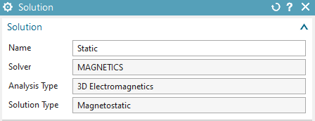
Name the solution ’Static’
Accept solver ’MAGNETICS’ and
analysis type ’3D Electromagnetics’,
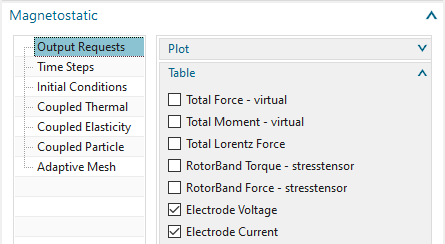
In the output requests, activate the tabular results ’Electrode
Voltage’ and ’Electrode Current’ to get tabular output for voltage and
current on the coils. This will allow us to compute the ohm resistance
by the formula \(R=U/I\).
Click OK.
Create a second solution (in the Sim part, use button ![]() )
of type ’Magnetodynamic Transient’.
)
of type ’Magnetodynamic Transient’.
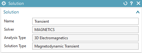
Name the solution ’Transient’
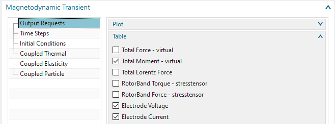
In the output requests ’Plot’, activate ’Magnetic Flux Density’
and ’Current Density’. In the ’Table’, activate ’Total Moment - entire
(virtual)’ to get tabular output of rotor torque over time steps. Also
activate ’Electrode Voltage’ and ’Electrode Current’.
Feel free to activate more results as desired.
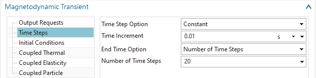
In register ’Time Steps’, set ’Number of Time Steps’ to 20 and
’Time Increment’ to 0.01 sec.
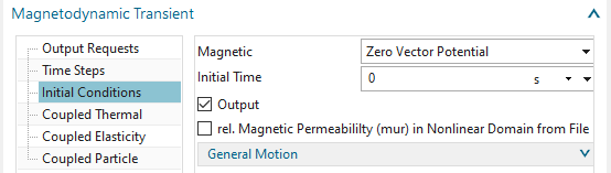
In register ’Initial Conditions’, activate ’Output’ to output the
results of time zero.
Click OK.
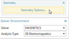
Set the Fem file to the displayed part.
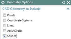
Edit the Fem file and activate ’Splines’ in Geometry
Options.
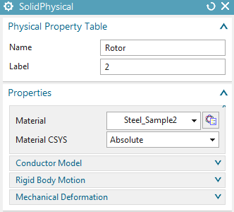
The Rotor
Mesh using tetrahedral elements with the half of the suggested element size (8.83/2 mm).
Apply material ’Steel_Sample2’ (From library
’Magnetics_Materials.xml’ in folder MAGNETICS). Notice that this
material has a nonlinear B-H curve. It contains the data of the TEAM24
task description.
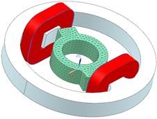
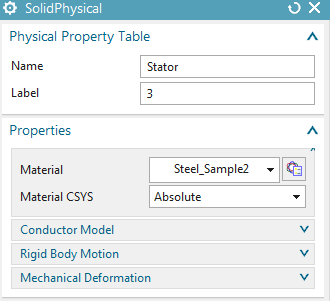
The Stator
Mesh with tets and half of suggested element size (14.6/2 mm).
Apply material Steel_Sample2.
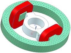
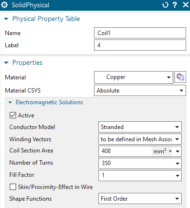
The first Coil
Mesh by tets and the suggested element size (8.92 mm).
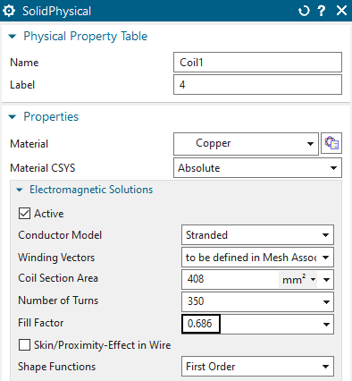
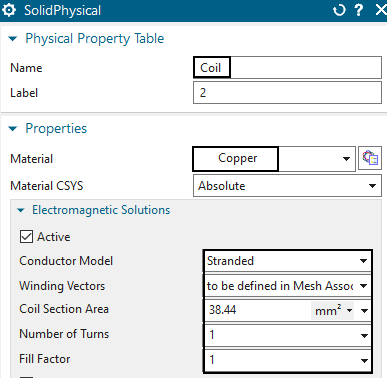
Name the physical ’Coil1’.
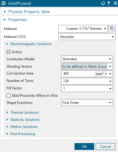
Set the material to ’Copper’. Make sure this copper has a electric conductivity (58e6 S/m).
Set the ’Conductor Model’ to ’Stranded’, use 350 Turns and a Section Area of 408 \(mm^{2}\).
Accept the default ’Fillfactor’ of 1. Later we will adapt this to
drive the coil to the demanded resistivity value.
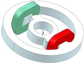
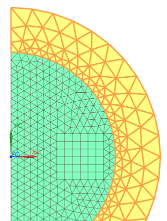
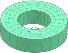
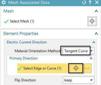
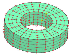
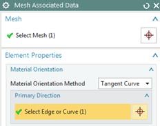
Edit the ’Mesh Associated Data’ of Coil1 mesh. Set the ’Electric
Current Direction’ option to ’Tangent Curve’ and select the spline curve
to define the direction of the windings.
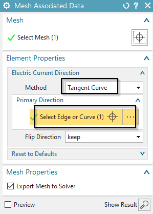
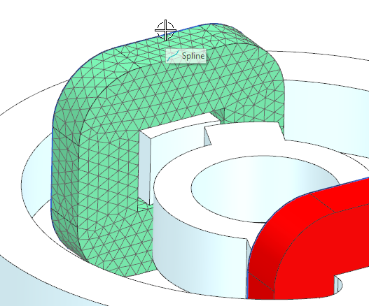
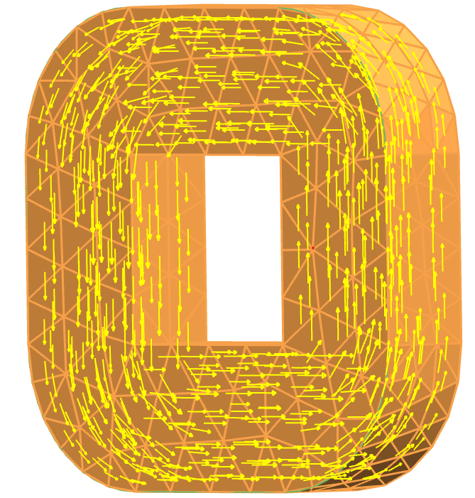
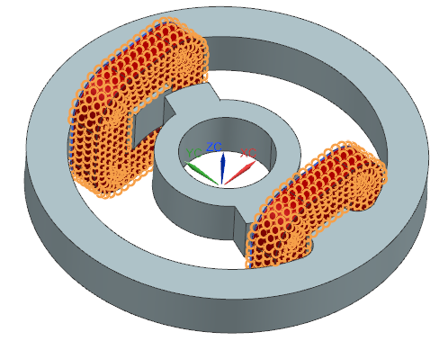
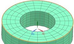
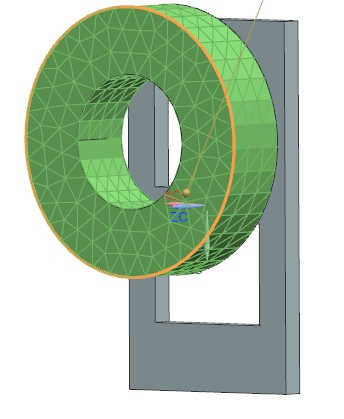
Hint: Activate ’Preview’ to check the winding direction. It
should look like the picture below.
The second coil
Use the same steps as for the first coil. Assign ’Coil2’ for name.
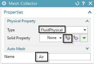
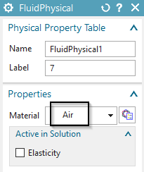
The Air:
Mesh the air volume with tets and use the suggested element size (34.5 mm).
Set the physical to ’FluidPhysical’ and assign material
Air.
For easier post processing, click on the button ’Rename Meshes
...’ ![]() from the Magnetics toolbar. That
utility renames all meshes and therefore is a useful feature especially
with larger models and many meshes.
from the Magnetics toolbar. That
utility renames all meshes and therefore is a useful feature especially
with larger models and many meshes.
Switch to the Sim file.
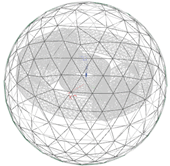
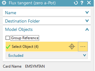
Create a constraint of type ’Flux tangent (zero a-Pot)’ on the
sphere outside faces.
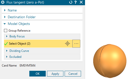
Create the voltage loads.
Apply voltage load of type ’On Stranded Coil’ on the first coil.
Assign 23.1/2 V.
Apply a second voltage on the second coil with the same value.
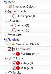
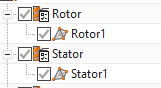
Assign these two loads and the constraint (by drag and drop) to
both solutions. The navigator should look like in the picture.
Prior to solving the static solution we must avoid that the coils are influenced by the rotor and stator. Therefore,
change to the Fem part,
drag and drop the meshes of the rotor and stator into the air
collector. Now these two will behave as air and not affect the
coils,
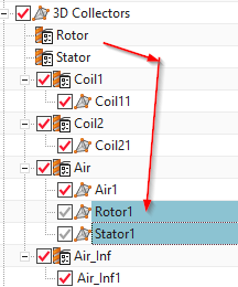
change back to the Sim part and solve the ’Static’ solution. The solution time should be about 0.5 minutes.
After the solve job has finished open the newly created afu- or
text file Team24_sim1-Static.globalcurrent.txt with the XY Function
Navigator or with a text editor. Find there the resulting current at the
two coil electrodes. The result is about 10.89 A.

According to \(R=U/I\) we can
compute the actual resistance to \(R=11.55 V /
10.89 A = 1.06 Ohm\). Because the demanded resistance is \(3.09/2 Ohm =1.545 Ohm\) the scale factor
becomes \(1.06 / 1.545 = 0.686\). To
use this factor as fillfactor switch to the Fem part and edit the two
physicals of the two coils. Set the ’Fillfactor’ as shown in the
picture:
Test solve again the static solution and find the new current
result as 7.47 A.

Now the resistance of the coil is R=11.55 V / 7.47 A = 1.54 Ohm as it is demanded in the Team task description.
Prior to solving the transient solution, move the two meshes of
rotor and stator back into their origin mesh collectors. Then solve. The
solution time will be about 3 minutes because of nonlinear iterations
due to saturation effects.
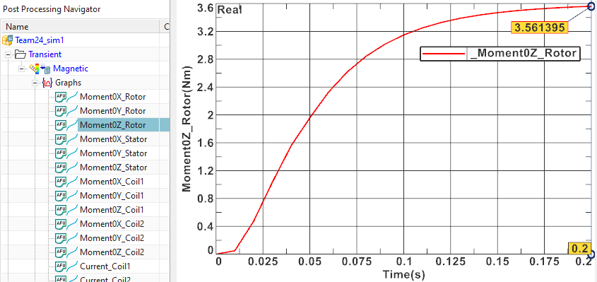
Check current and torque results over time.
Open the graphical table results and display them as follows.
Display z component of the torque on the rotor. The maximum value
is 3.56 Nm. The reference result from measurements is 3.2 Nm. Smaller
mesh sizes will drive the simulation result more and more against the
measurement.
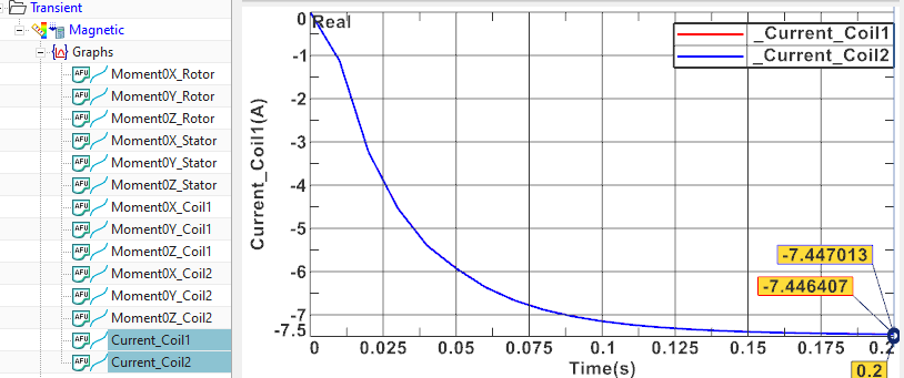
Display the current result for both coils. They show a good
agreement and the maximum value is 7.45 A. The measured reference value
for the current is 7.4 A at time 0.2 sec.
A manual verification of the time dependent current \(I(t)\) in a coil after switching on the
voltage, is given by the formula: \[I(t) =
(1-e^{\frac {R}{L} \cdot t}) \cdot \frac{U_{0}}{R}\]
with \(R = 1.54 \Omega\), \(L = 0.03H\), \(U_{0} = 11.55V\) and \(t = 0.01s, ..., 0.2s\).
L is precalculated by the formula: \[L
\approx \mu_r \cdot \mu_0 \cdot N^2 \cdot \frac{A}{l} \approx
0.03H\]
Following a table with a comparison of the simulation and analytic
results:
| Time | Simulation Result | Analytic Result | Deviation | |
|---|---|---|---|---|
| 0.01s | 2.65A | 3.01A | \(13.6\%\) | |
| 0.05 | 6.2A | 6.92A | \(11.6\%\) | |
| 0.1s | 7.2A | 7.45A | \(3.5\%\) | |
| 0.15s | 7.38A | 7.49A | \(1.5\%\) | |
| 0.2s | 7.43A | 7.4997A | \(0.9\%\) |
The values match well at the end time. Deviations in the beginning are
higher probably because of the unsecure inductivity value of the
coils.
The contour plot of the flux density at time 0.2 s (last time
step) looks like this:
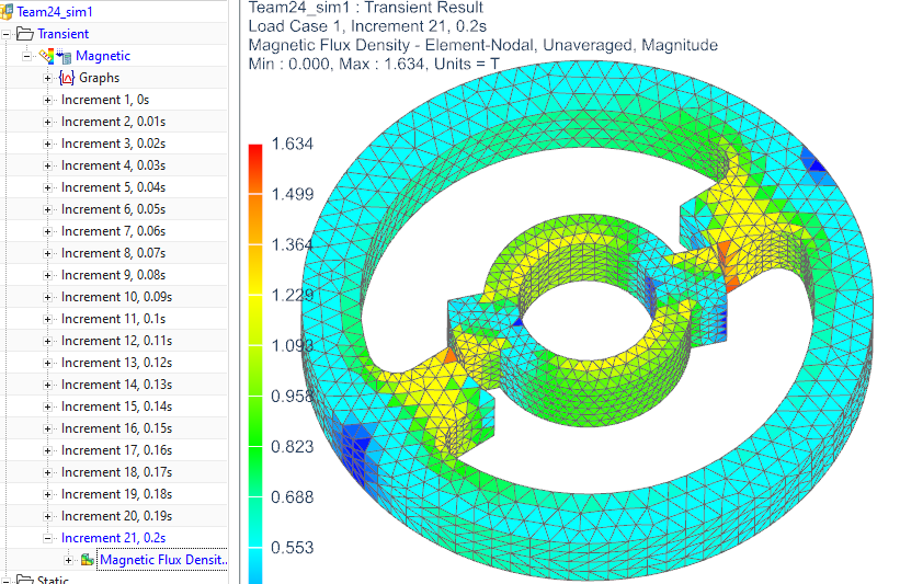
The tutorial is finished.
In this example we show how to calculate inductance, ohm resistance,
voltage, current and their phase shift in a simple coil. We start with a
1D simulation where we assign the values of current, inductivity and
resistance. The simulation calculates the resulting voltage. In a
similar way one could also set up much more complex electrical circuits
and compute for such results. Following we simulate this in a 2D
axisymmetric and also a 3D simulation. The advantage of 2D and 3D
simulation is that the parameters of the coil are calculated with the
given geometry by FEM. Another possibility is to combine 1D circuits
with 2D and 3D models, what is not shown in this tutorial.
Estimated time: 1 h.
Start the Program Simcenter ![]() (or
NX). Use Version 10 or higher.
(or
NX). Use Version 10 or higher.
Create a new .prt file.
Start the application Pre/Post.
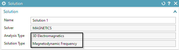
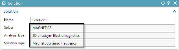
Choose solver ’MAGNETICS’ and Analysis Type ’3D Electromagnetics’(’2D or axisym Electromagnetics’ is also possible). Click OK.
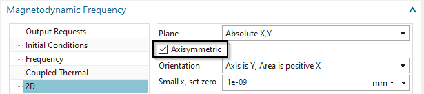
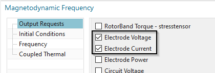
Set Solution Type to ’Magnetodynamic Frequency’.
In register ’Output Requests’ under ’Table’ activate ’Circuit Voltage’.
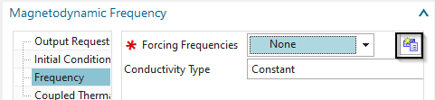
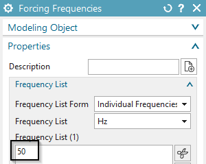
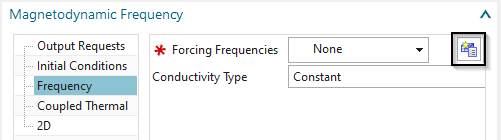
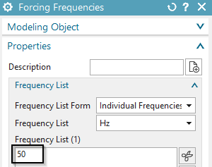
In register ’Frequency Domain’, create a modeling object and set
the ’Forcing Frequency’ to 50 Hz(Picture below).
Switch to the Fem-file.
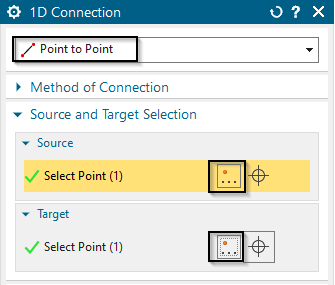
From toolbar ’Home’ create a ’1D Connection’
Switch from ’Node to Node’ to ’Point to Point’
In ’Source’ open the ’Point Dialog’ and key in ’100’ for the X coordinate. Accept ’0’ for Y and Z. Do the same in ’Target’ with X = 100, Y = 100, Z = 0. (Any other coordinates are possible)
Under ’Element Properties’ switch to ’Inductor’.
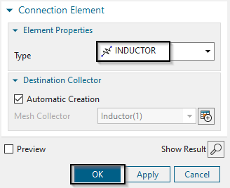
Click OK. There now appears a symbol of the inductor between the two points.
In the Simulation Navigator double click on the created mesh collector ’Inductor(1)’.
Click edit.
In ’Normal Values’ key in ’1’ H.
Create again a 1D Connection.
As ’Source’ use the first Point. As ’Target’ create a new point with X = 100, Y = 200, Z = 0.
Switch the type of the ’Connection Element’ to ’Resistor’. Click OK. The symbol of the resistor is a straight line.
Edit the properties of the resistor. Type ’1’ \(\Omega\) in ’Electric Resistance per Element’.
Switch to the Sim-file.
Create a new Load. Use ’Current Harmonic’.
Switch from ’On Stranded Coil’ to ’On Circuit’
For the ’Primary Node’ select the point at the bottom of the inductor. For the ’Secondary Node’ select the point on top of the resistor.
The ’Electric Current Amplitude’ is set to ’3’A.
Click RMB on the Solution, select ’Edit Solver Parameters’ and under ’Result Graphs(afu) switch to ’Create, keep txt Files’. Solve the Solution.
Postprocessing is done by some text or afu files that contain the results.
Open the file with extension *.VoltageCircuits.txt. The Solution
is divided in the applied voltage, the ’Inductor Element’ and the
’Resistor Element’. Each has three parameters. The first is the
frequency following the real part and last the imaginary part.

Applied voltage: real part = 3V, imaginary part = 942.48 V.
Inductor: real part = 0 V, imaginary part = 942.48 V.
Resistor: real part = 3 V, imaginary part = 0 V.
Impedance of the inductor: \(Z_{L} =
U/I = (0V + j942.48V)/3A\)
Impedance of the resistor: \(Z_{R} = U/I = (3V
+ j0V)/3A\)
Impedance of circuit : \(Z_{RL} = Z_{L} +
Z_{R} = 1 \Omega +j100 \pi \Omega\)
For the calculation of the voltage in the coil we need the ’reactive’
resistance of the coil \(X_{L}\). This
is calculated by: \[X_{L} = j \omega L = j
\cdot 2 \pi \cdot f \cdot L = j100 \pi\] with \(f=50Hz\) forcing frequency, \(L=1H\) inductivity of coil.
To calculate the voltage we use \(U = X_{L}
\cdot I = j100 \pi \cdot 3A = 942.478V\)
The resistance of the resistor was set to \(R
= 1 \Omega\).
So the voltage in the resistor is \(U = R
\cdot I = 1 \Omega \cdot 3A = 3V\)
These results match with the results of the simulation.
download the model files for this tutorial from the following
link:
https://www.magnetics.de/downloads/Tutorials/4.MagDyn/4.4Coil.zip
unzip the archive. There will be one folder ’start’ and one ’complete’.
Start the Program Simcenter ![]() (or
NX). Use Version 10 or higher.
(or
NX). Use Version 10 or higher.
In Simcenter, click Open ![]() and navigate to folder ’start’. Select
the file ’coil2D.prt’ and click OK. (Maybe you must set the file filter
to ’prt’)
and navigate to folder ’start’. Select
the file ’coil2D.prt’ and click OK. (Maybe you must set the file filter
to ’prt’)
Start the application Pre/Post.
Create a New Fem and Sim. Set the solver to ’MAGNETICS’ and Analysis Type ’2D or axisym Electromagnetics’. Click OK.
A new window appears asking for the solution type. See below.
Set the Solution Type to ’Magnetodynamic Frequency’.
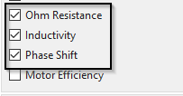
In register ’Output Requests’, ’Table’ activate ’Ohm Resistance’,
’Coil Inductivity’ and ’Phase Shift’,

In register ’Frequency’ create a modeling object for ’Forcing
frequencies’ with 50 Hz.
In register ’2D’ activate ’Axisymmetric’ and click OK.
Switch to the FEM file.
Mesh the conductor face using quad elements and the suggested element size /2.
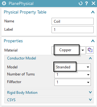
Assign ’Copper’ material and set the ’Conductor Model’ to
’Stranded’.
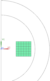
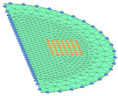
Mesh the air face using tri elements (half of suggested size) and assign ’Air’.
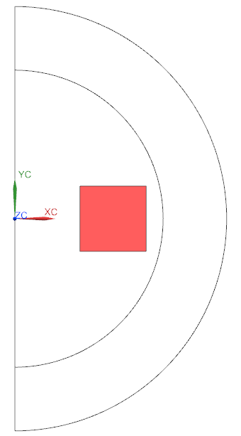
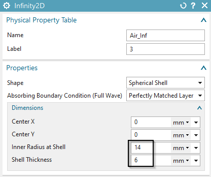
Mesh the Infinity area with tri elements (suggested element
size). Assign a physical of type ’Infinity2D’ and use the dimensions as
shown in the picture.
For easier post processing, click on the button ’Rename Meshes
...’ ![]() from the Magnetics toolbar. That
utility renames all meshes and therefore is a useful feature especially
with larger models and many meshes.
from the Magnetics toolbar. That
utility renames all meshes and therefore is a useful feature especially
with larger models and many meshes.
Switch to the Sim file.
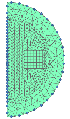
Create a Constraint of type ’Flux tangent (zero a-Pot’ at the
middle axis and on the circular border.
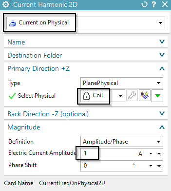
Create a Load of type ’Current Harmonic 2D’ with type ’Current’
on the conductor face. Assign an Electric Current of 1 A and a Phase
Shift of zero deg.
Under Solution, select ’Edit Solver Parameters’ and modify the field Result Graphs (afu) to ’Create, keep txt Files’.
Solve the solution.
Check the flux density result. (real part)
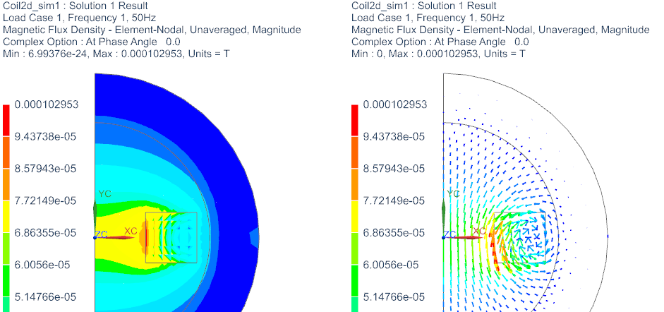
Postprocessing is done by some text or afu files that contain the results.
Ohm-Resistance Result
Open the file with extension *.ohmresistance.txt. There are two results for each region. The first one is the ’Active Resistance’ (Wirkwiderstand) and the second is the ’Reactive Resistance’ (Blindwiderstand). The resistance is derived from the voltage and current results by \(R=U/I\). On region ’Current(1)’ the result is
’Active Resistance’: \(2.6\mathrm{e}{-5}\) Ohm
’Reactive Resistance’: \(4.9\mathrm{e}{-6}\) Ohm .
This result is valid for a coil with one winding. For a coil with
N windings you can set the ’Number of Turns’ in the conductor properties
to the desired N. Alternatively the result values can be multiplied by
\(N^{2}\).

Inductance Result
Open *.inductivity.txt.
The Inductance is derived from the voltage and current results by
\(L=(U/I)/(2Pi*f)\). On region ’Coil’
the result is \(1.57\mathrm{e}{-9}\)
Henry. Again this result is valid for a coil with one winding. For a
coil with N windings the result value has to be multiplied by \(N^{2}\).

Phase Shift Result
Open *.phase.txt.
The phase shift is derived from voltage results by \(Phi=arctan(U_{imag}/U_{real})\). On region
’Coil’ the calculated phase shift is 6 deg. This result does not depend
on the number of windings.

Open the part ’coil3d.prt’,
Start Simcenter Pre/Post, Create New FEM and Sim,
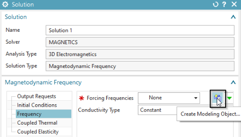
Choose solver ’MAGNETICS’ and Analysis Type ’3D Electromagnetics’.
Set Solution Type to ’Magnetodynamic Frequency’.
In register ’Output Requests’ under ’Table’ activate the shown
options
In register ’Frequency Domain’, create a modeling object and set
the ’Forcing Frequency’ to 50 Hz.
Switch to the Fem-file.
Create Mesh-Mating Conditions.
Hex-mesh the coil: Use the half of the suggested element-size
(4.62/2 mm). Assign material ’Copper’ and the settings as shown in the
next picture.
Assign vectors to the coil mesh.
Tet-mesh the air: Use the suggested element-size (4.92 mm). Hint: Activate the ’Pyramid Transition’ option for correct transition between hex and tet elements.
Assign material ’Air’.
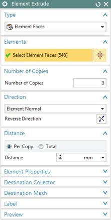
Use the function ’Extrude’ from toolbar ’Nodes and Elements’ to
create 3 layers of infinity elements. Use a distance of 2 mm for each
layer. Insert the settings to the Infinity physical as shown in the
picture.
Switch to the Sim-file
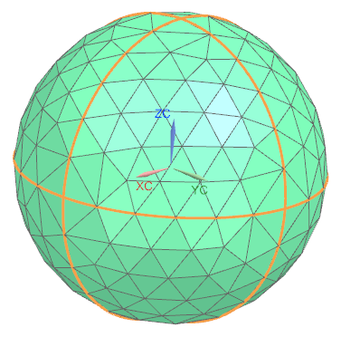
Create a constraint ’Zero Potential - Flux tangent’ on the outside element-faces of the sphere.
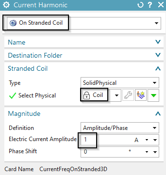
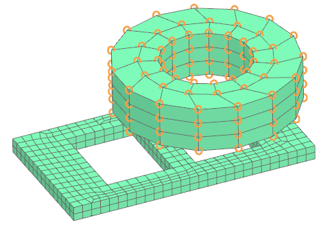
Create a load of type ’Current Harmonic’ on any of the faces of
the coil. Assign 1 A and zero phase shift.
Under Solution, select ’Edit Solver Parameters’ and modify the field Result Graphs (afu) to ’Create, keep txt Files’
Solve the solution
Postprocessing is done by some text files that contain the results.
Voltage Result
Open *.globalvoltage.txt .
There are two values for each region. (the very first value is the forcing frequency) The first is the calculated ’Active Voltage’ (Wirkspannung) and second is the ’Reactive Voltage’ (Blindspannung). On region ’Coil’ the result is
’Active Voltage’ (Wirkspannung): -2.58e-5 V
’Reactive Voltage’ (Blindspannung): -4.66e-6 V .

Current Result
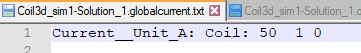
Open *.globalcurrent.txt.
Again there are two results for each region. The first is the
’Active Current’ (Wirkstrom) and the second is the ’Reactive Current’
(Blindstrom). Because in our example we have a series circuit
(Reihenschaltung) of inductivity and ohm-resistance the reactive current
has to be zero. The sum of all active currents has to be zero, region
’Coil’ has 1 Ampere.
Ohm-Resistance Result
Open *.ohmresistance.txt.
Again there are two results for each region. The first one is the ’Active Resistance’ (Wirkwiderstand) and the second is the ’Reactive Resistance’ (Blindwiderstand). The resistance is derived from the voltage and current results by \(R=U/I\).
This ohm resistance result is valid for a coil with one winding.
For a coil with N windings the result values have to be multiplied by
\(N^{2}\).

Inductance Result
Open *.inductivity.txt.
Again there are two results for each region, but in this case the second one does not have a meaning. The Inductance is derived from the voltage and current results by \(L=(U/I)/(2Pi*f)\).
This result is valid for a coil with one winding. For a coil with
N windings the result value has to be multiplied by \(N^{2}\).

Phase Shift Result
Open *.phase.txt.
Again there are two results for each region, but in this case the
second one does not have a meaning. The phase shift is derived from
voltage results by \(Phi=arctan(Uima/Ureal)\).

For approximate analytic calculation of the inductance \(L\) of an air-coil, we use the following
formula (Source: G. Schenke, Bauelemente der Elektrotechnik 2008, S.
37.) \[L \approx \mu_0 N^2 0.51 D_{out} =
1.589 \cdot 10^{-8} H\] with \(D_{out}=0.0248 m\): Diameter of coil, \(N=1\) Number of turns, \(\mu_0=4 \pi 10^{-7}\) Magnetic
constant
The active ohm resistance \(R\) (Re
part) can be calculated from the length \(l\) and section area \(A\) of the wire and the electric
conductivity \(\sigma\) as \[R = \frac{l}{\sigma A} = 2.62 \cdot 10^{-5}
\Omega\] with \(\sigma=58 \cdot 10^6
S/m, l=0.058m, A=3.8438 \cdot 10^{-5} m^2\)
The reactive ohm resistance \(XL\) (Im
part) can be calculated from the inductance \(L\) and the frequency \(f\) from \[XL =
\omega L = 2 \pi \cdot f \cdot L = 4.99\cdot 10^{-6} \Omega\]
with \(f=50Hz, L=1.589\cdot 10^{-8}
H\).
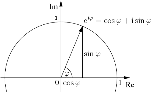
The phase shift \(\varphi\) results
from the two resistance values by \[\varphi =
\arctan \frac{Im}{Re} = 10.7 deg\]
Finally, an overview of the calculated results in 2D and 3D and analytic
is shown.
| Ohm Resistance (active) | Ohm Resistance (reactive) | Inductance | Phase Shift | |
|---|---|---|---|---|
| Analytic | \(2.62 \cdot 10^{-5} \Omega\) | \(4.99 \cdot 10^{-6} \Omega\) | \(1.589 \cdot 10^{-8} h\) | \(10.7 \deg\) |
| 2D | \(2.614 \cdot 10^{-5} \Omega\) | \(4.938 \cdot 10^{-6} \Omega\) | \(1.572 \cdot 10^{-8} h\) | \(10.698 \deg\) |
| 3D | \(2.581 \cdot 10^{-5} \Omega\) | \(4.658 \cdot 10^{-6} \Omega\) | \(1.483 \cdot 10^{-8} h\) | \(10.23 \deg\) |
As another reference, the benchmark example ’TEAM 15’ gives an inductance value for a similar coil with N=3790 windings as \(0.2218 h\). In our 2D example we calculated \(0.2258 h\). Thus, the deviation in 2D is 1.8% and in 3D 4%.
The exercise is done. Save your files and close them.
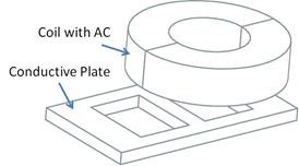
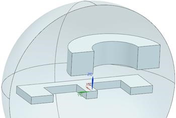
The problem 3 of the Team Benchmarks (Testing Electromagnetic
Analysis Methods) is one of the examples for testing eddy current
effects. A conductive plate with two holes is placed under a coil. The
coil is driven by alternating current of 50 Hz and 1260 ampere turns.
The goal is to analyse for the magnetic flux density along a line that
goes slightly over the plate. The user should read the documents
’problem3.pdf’ and ’Results_EddyCurrentProblems.pdf’ for more background
understanding.
What you learn in this example:
Perform 3D Magnetodynamic analysis in frequency domain,
Display and calculate the Skin depth.
Estimated time for the example: 1h.
Follow these steps:
download the model files for this tutorial from the following
link:
https://www.magnetics.de/downloads/Tutorials/4.MagDyn/4.3Team3.zip
unzip the archive. There will be one folder ’start’ and one ’complete’.
Start the Program Simcenter ![]() (or
NX). Use Version 10 or higher.
(or
NX). Use Version 10 or higher.
In Simcenter, click Open ![]() and navigate to folder ’start’. Select
the file ’Team3_full.prt’ and click OK. (Maybe you must set the file
filter to ’prt’)
and navigate to folder ’start’. Select
the file ’Team3_full.prt’ and click OK. (Maybe you must set the file
filter to ’prt’)
From toolbar Application click on ’Pre/Post’ ![]()
Click in toolbar ’Magnetics’ on ’New FEM and Simulation
(Non-Manifold)’ ![]() .
.
Create a new Solution
Accept the Solver ’MAGNETICS’ and choose the Analysis Type ’3D Electromagnetics’,
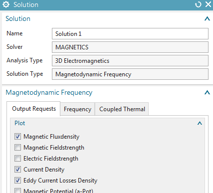
Choose Solution Type ’3D-Magnetodynamic Frequency’
In register ’Output Requests’, ’Plot’ set ’Current Density’ and
’Eddy Current Losses Density’ on to compute eddy current effects.

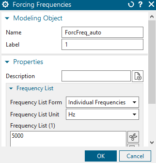
In register ’Frequency Domain’, click ’Create Modeling Object’.
In the following window ’Forcing Frequencies’, key in 5000 Hz into the
list and click OK.
Set the displayed part to the Fem-file.
The Coil:
Create a 3D tetra mesh on the coil body. Select the coil, key in the source element size (half of the suggested). Click OK.
Edit the physical of the coil and assign the material Copper to it.
Set the ’Conductor Model’ option to ’Stranded’. The ’Number of
Turns’ to 126 and the ’Coil Section Area’ to \(400 mm^{2}\).
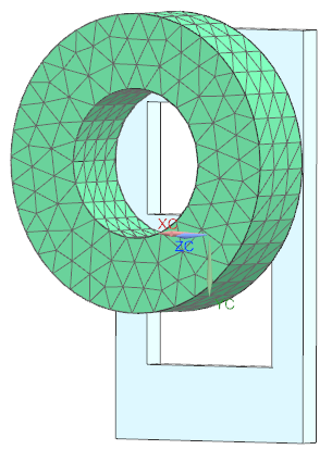
Edit the Mesh Associated Data for the coil mesh. Set the
’Material Orientation’ to ’Tangent Curve’ and select the circular edge
to describe the winding direction.
The Plate:
Create a 3D tetra mesh on the plate. Use the system suggested value/4.
Edit the physical and click ’Choose Material’![]() .
.
Click on ’Create Material’ (Bottom right)![]() .
.
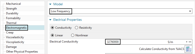
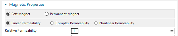
Under ’View’, switch to ’All Properties’. As name, type in ’PlateSample’.
Under ’Electromagnetics’ set ’Model’ to ’Low Frequency’.
For ’Electrical Conductivity’, type in \(32760000 S/m\). And for ’Relative
Permeability’, key in 1. Click OK several times until the window
disapears.
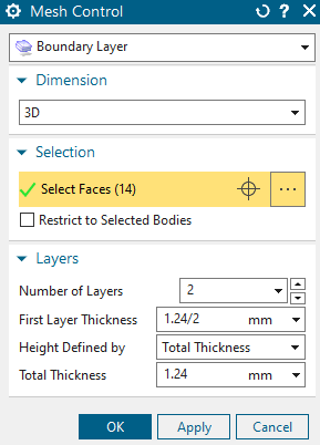
Mesh Control
Click on ’Mesh Control’ ![]() .
.
Assign ’Boundary Layer’
Select all plate faces (drag a window).
Under ’Number of Layers’, key in 1, ’First Layer Thickness’, 1.24
and ’Total Thickness’, 1.24. We do this to consider the skin depth in
this simulation. Click OK.
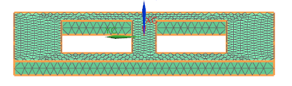
Hint: Because of the skin effect, eddy currents will appear mainly at
the border of the conductor. The thickness of that eddy current layer is
called Skin Depth. For a accurate simulation this skin depth should be
meshed with high quality elements. At least one layer of elements as we
do in the following. The skin depth (\(\sigma\)) can be calculated by the formula:
\[\delta = \frac{1}{\sqrt{\pi \cdot f \cdot
\mu_0 \cdot \mu_r \cdot \sigma }} = 1.24 mm\]
with \(f = 5000Hz\), \(\mu_0 = 4\pi \cdot 10^{-7}\), \(\mu_r = 1\), \(\sigma = 32760000\) S/m.
Update the FEM![]() .
.
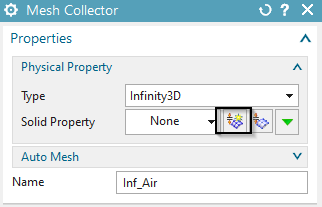
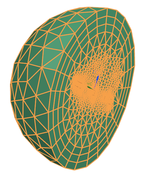
The Air
Create a 3D tetrahedral mesh with the suggested size (24.1 mm) on the air volume. Use the existing mesh collector ’AIR (3d)’.
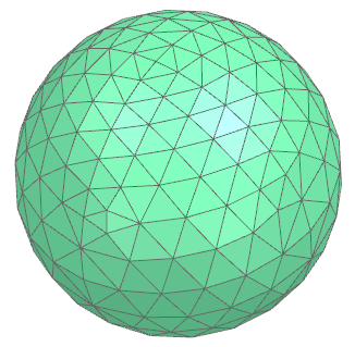
The Air Infinity
This step is optionally for higher result accuracy but it can only be done if there is a geometry for the infinity air (not the case in the geometry file): Create a 3D tetrahedral mesh and select the body ’AirInf’ (not available in current model but can be created in the prt file) and accept the suggested size. Activate ’Automatic Creation’. Click OK.
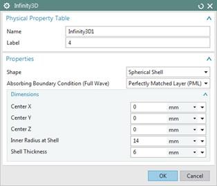
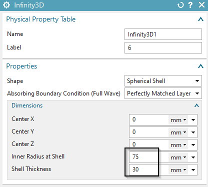
Create for this mesh a physical of type ’Infinity3D’ and
Insert the settings into the physical as shown.
Switch to the Sim-file
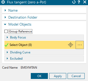
Create a constraint of type ’Flux tangent (Zero-a-Pot)’ on the
outside element faces of the Air Infinity sphere. Set the selection
filter to ’Tangent Faces’ and select a face. Click OK.
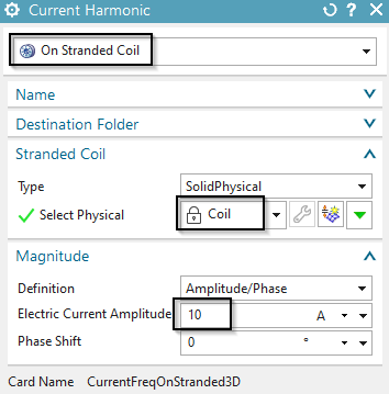
Create a load ’Current Harmonic’ with type ’On Stranded Coil’ on
the coil. Assign 10 A.
Solve the solution. The solution time is about 1 minute.
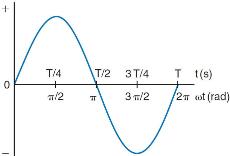
In all frequency domain solutions results are complex, that means they have a real (Re) and an imaginary (Im) part. One can imagine the corresponding time domain solution would alter between this real and imaginary part. From real and imaginary part other quantities like amplitude and phase angle can be extracted by complex number math operations.
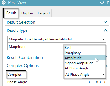
Hints for viewing frequency results in post processing:
All frequency results are available in complex format what means
the NX postprocessor can handle these comfortably. The ’Complex Options’
can be set by first clicking ’Result’ ![]() and
then modifying the ’Complex’. That allows to switch between ’Real’,
’Imaginary’, ’Amplitude’ and ’At Phase Angle’.
and
then modifying the ’Complex’. That allows to switch between ’Real’,
’Imaginary’, ’Amplitude’ and ’At Phase Angle’.

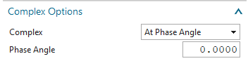
The complex results of frequency solutions can be shown as time results. To do so, an animation over the ’Phase Angle’ must be done. This will show, step by step, how the real part changes to the imaginary part, thus, the corresponding time solution. Proceed as follows:
Set the option ’Complex’ to ’At Phase Angle’.
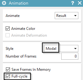
Click ’Animation’ ![]() and set the ’Style’ to ’Modal’.
Activate ’Full Circle’. Then click ’Play’. The animation will show the
corresponding time result.
and set the ’Style’ to ’Modal’.
Activate ’Full Circle’. Then click ’Play’. The animation will show the
corresponding time result.
In the ’Post Processing Navigator’ double click on the ’Current Density’ result.
Hide the 3D elements Coil, Air, AirInf and all 2D elements.
Current Density Result:
The picture shows the area where the eddy currents appear. It
corresponds to the prior calculated skin depth.
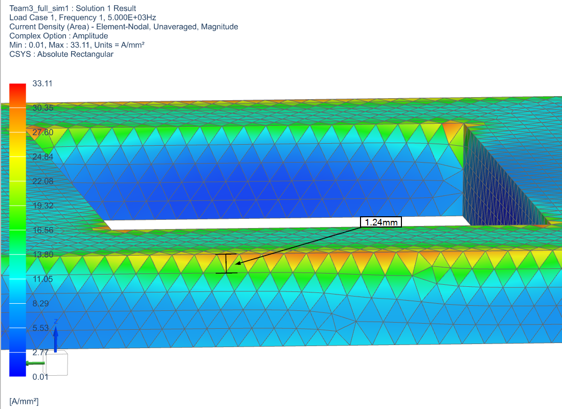
The picture shows the area where the eddy currents appear.
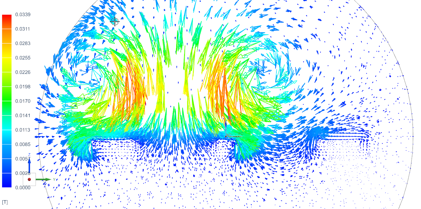
Flux density plot with arrows and the ’Complex Option’ is set to
’At Phase Angle’. Visible is the magnetic field, created by the coil and
influenced by the plate.
EddyCurrentLossesDensity:
This result is responsible for the heating of the plate.
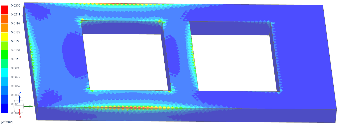
This result is responsible for the heating of the plate.
In this second part of the exercise we will demonstrate how conducting sheets can be used. Therefore, the aluminum plate will be modeled by 2D elements which take into account thickness and magnetic/electric material properties. This assumption is valid and of good accuracy if thickness is small. The model is already set up, so in this tutorial we simply walk through the steps and check the new features.
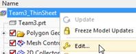
Open the part ’Team3_sim2.sim’ from the complete folder and
change to the FEM file. The part already contains a coarse mesh,
physical properties and boundary conditions for this exercise.
Set the Fem file to the displayed part.
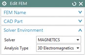
Edit the FEM file and verify the solver is set to MAGNETICS and
the analysis type is ’3D Electromagnetics’.
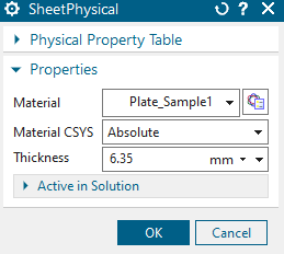
Notice the plate is meshed by 2D elements. The mesh resides in a
collector named ’PlateThin’. Check the physical of the plate. It is of
type ’SheetPhysical’ and materials and thickness properties are defined
as shown in the picture below:
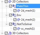
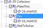
Notice that in this example we used a ’Solid from Shell Mesh’ for the air. Therefore, a ’Surface Coat Mesh’ on all 3D parts exists (collector ’NotToSolver’) and a tri mesh on the air boundary (collector ’Env’).
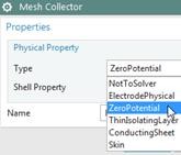
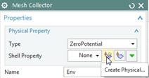
Check the 2D mesh collector ‘Env’. It contains a physical of type
ZeroPotential’ for the boundary. This physical has the same effect as a
constraint of type ’Flux tangent (zero a-Pot)’ in the Sim file. You can
use this alternatively. Its advantage is a little more performance when
writing out the solver input file.
Check the physical for the coil mesh. All properties are set in the same way as in the first part of this example (126 turns, \(400mm^{2}\) section area). Also the definition of the winding directions is already there.
Check the FluidPhysical for the air mesh.
Change to the Sim file.
The solver is Magnetics, Analysis type is 3D and Solution Type is
’Magnetodynamic Frequency’. All settings are set in the same way as in
the first part of this example.
The same current (10 A) is applied on the coil.
There is NO ’Flux Tangent (zero a-Pot)’ condition in the SIM file, because there is already a ZeroPotential physical that has the same function.
Solve and post process the results.
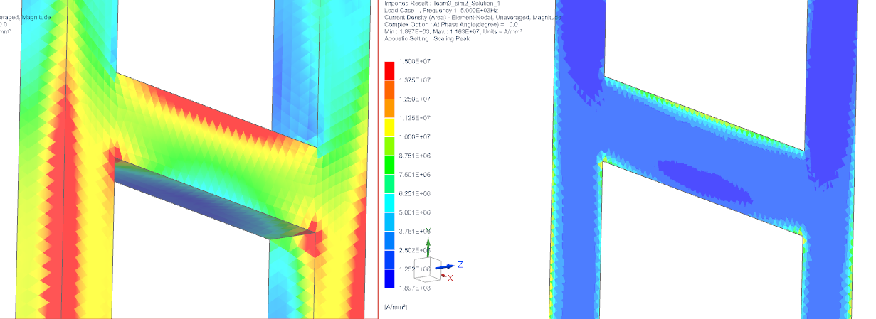
Check Current Density in comparison of the 3D plate with the 2D
sheet: See next picture (left 3D plate, right 2D sheet):
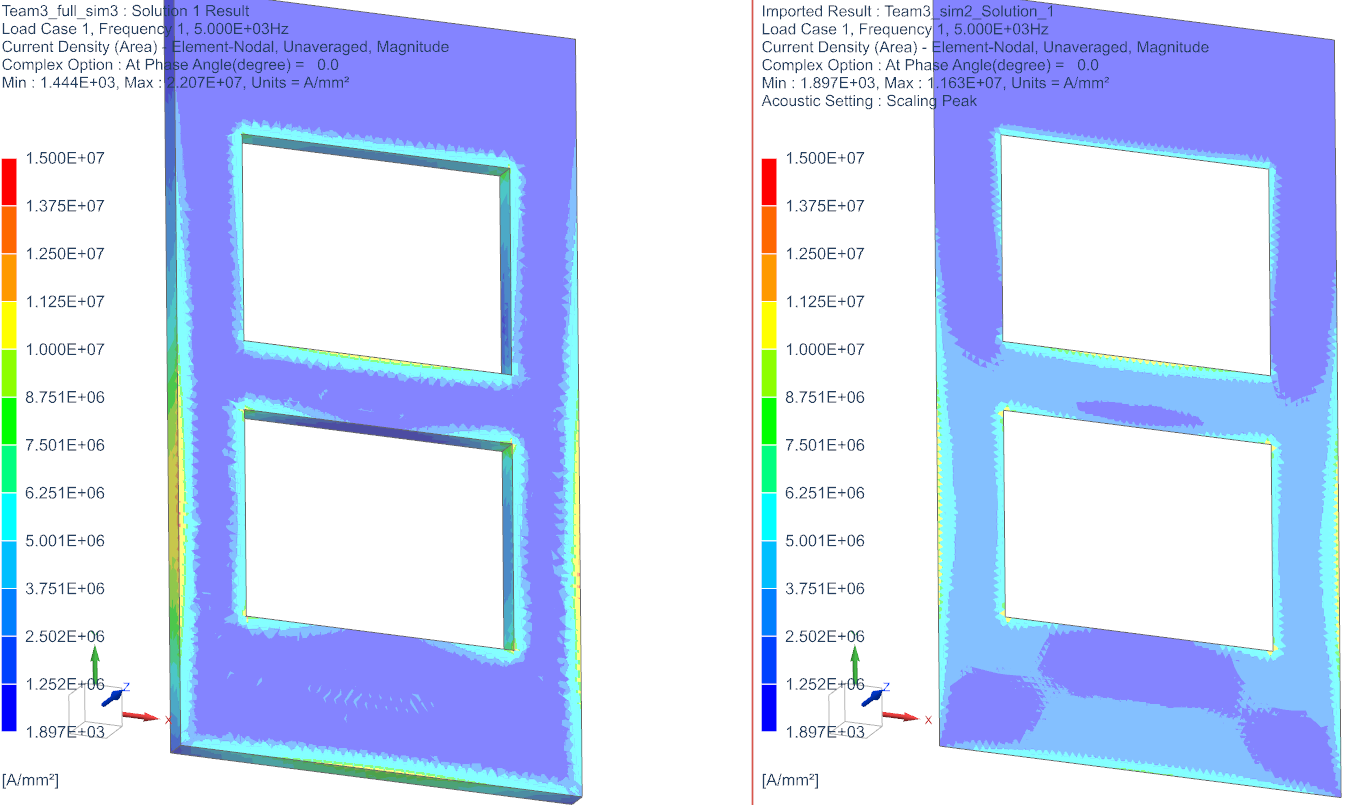
The overall agreement is ok, but notice there are deviations
between the 3D and the thin sheet results that result from edge effects.
The 3D results are more precise. The skin effect is more detailed using
the 3D plate model. Deviations become smaller with thinner plates.
In case the model and also the magnetic field are symmetric, the
simulation can be simplified. We use a half model and apply a symmetry
constraint on the symmetry plane.
The condition ’Flux tangent (zero a-Pot)’ on the symmetry plane acts as
a symmetry condition. Therefore, that condition has to be defined on all
outside faces: The outside sphere faces and the symmetry plane.
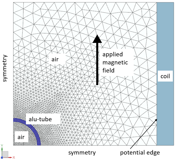
In this example an aluminum tube (depicted blue in the figure) will
be considered that is loaded by a time dependent magnetic field in
vertical direction. We will compute the time dependent induced current
(eddy current) within the tube. Such eddy current losses can then be
used to calculate temperatures on the tube (not shown in this tutorial).
Reference results are available from the TEAM benchmark. Additionally,
the reader may also read the attached document for the TEAM 1a task to
find further information.
According to the TEAM 1a description, the applied magnetic field
strength in the y direction decays exponentially with time as \[B_{y} = B_{0} \space e^{\frac{-t}{\tau}}\]
where \(B_{0} = 0.1 T\) and \(\tau = 0.0397\).
For this example we will apply the demanded magnetic field in two
different ways: first, we will apply said field via a difference of a
magnetic potential on the two opposing boundaries; and second, we will
apply an electric current on the coil face. In both cases the result
shall be very similar. In order to start from a steady state solution we
will first analyse for statics and then restart from this solution.
Estimated time for this example: 0.5 h
Exercises are:
Analysis of Eddy Currents, conductive and hysteresis Losses,
Symmetry constraints,
Applying given potentials as math function,
Using a steady state solution as initial condition.
download the model files for this tutorial from the following
link:
https://www.magnetics.de/downloads/Tutorials/4.MagDyn/4.1Team1a.zip
unzip the archive. There will be one folder ’start’ and one ’complete’.
Start the Program Simcenter ![]() (or
NX). Use Version 10 or higher.
(or
NX). Use Version 10 or higher.
In Simcenter, click Open ![]() and navigate to folder ’start’. Select
the file ’Team1a.prt’ and click OK. (Maybe you must set the file filter
to ’prt’)
and navigate to folder ’start’. Select
the file ’Team1a.prt’ and click OK. (Maybe you must set the file filter
to ’prt’)
Start application Pre/Post and create a ’New Fem and Sim’ File.
Set off the creation of an Idealized Part.
Choose the Solver ’MAGNETICS’, ’2D or axisym Electromagnetics’.
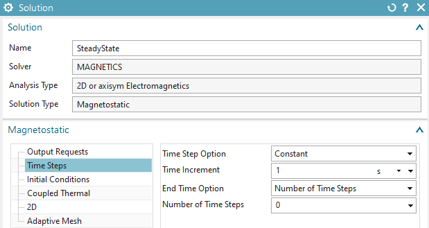
Create a Solution of type ’Magnetostatic’.
Hint: This will be the steady state solution that we will later use to
restart from.
Name the solution ’SteadyState’.
In register ’Time Steps’, accept the defaults ’Number of Time
Steps’ as 0 as well as ’Time Increment’ as 1.
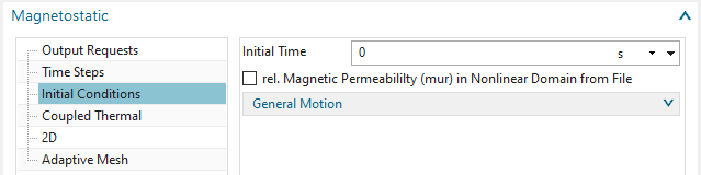
In register ’Initial Conditions’, accept the defaults, i.e.
’Initial Time’ to 0 s.
Hint: A second solution will restart from this first solution.
Therefore, we want the second solution to start at time 0; meaning that
we have to use zero time for this first solution.
Accept all other default settings.
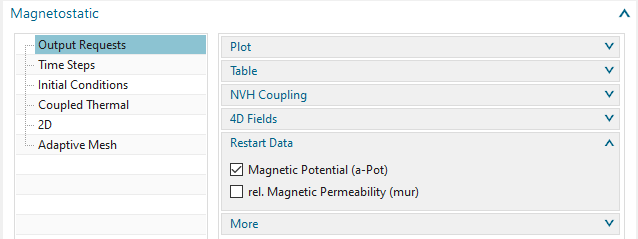
Edit the output requests of this solution. In box ’Restart Data’,
activate ’Magnetic Potential (a-Pot)’.
Hint: This setting is necessary to use this solution later to restart
from.
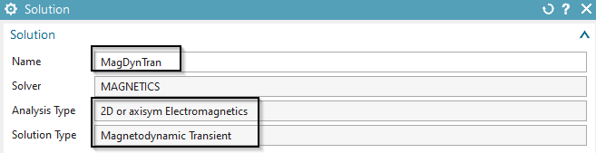
Create a second solution of type ’Magnetodynamic Transient’. Name
it ’MagDynTran’. Hint: This will be the main solution
Activate the following Output Requests in register ’Plot’:
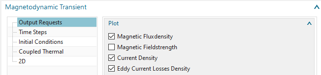
’Current Density’: To compute the induced eddy currents and display them as a contour plot.
’Eddy Current Losses Density’: To compute the losses \(P_{c}\) that result from electric resistance and eddy currents \(I\) corresponding to \(P_{c} = R I^{2}\) with R as ohm resistance. This approach for losses analysis is valid typically in massive conductors where hysteresis effects are neglectable.
And in register Table:
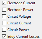
’Eddy Current Losses’: To compute the losses \(P_{c} = R I^{2}\) integrated over geometry
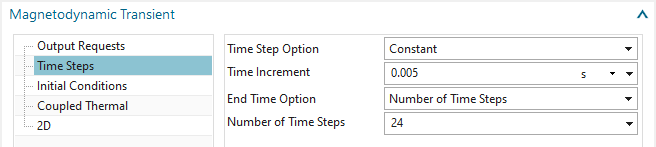
Set the ’Time Steps’ settings as in the next picture
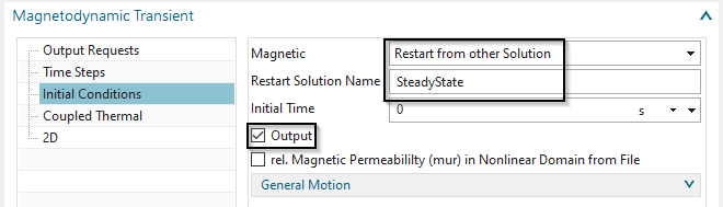
In register ’Initial Conditions’: Set the option
’Magnetic/Temperature’ to ’Restart from other Solution’. Key in the name
of the already created solution into the field ’Restart Solution Name’.
Also activate ’Output’ to enable the system to write the results for the
initial condition to the result file. This is for checking only.
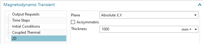
Accept the defaults in register ’2D’. Ok.
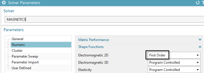
To avoid a sharp step of eddy currents that would appear at the
beginning: In solver parameters under ’Numeric’, set the option ’Shape
Functions, Electromagnetic’ to ’First Order’.
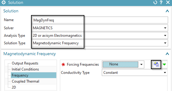
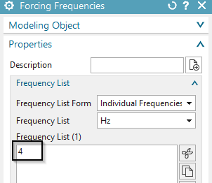
Optionally step: This problem can also be solved in frequency
domain. The excitation has a frequency of about 4 Hz. So, if desired,
create another 2D solution of type ’Magnetodynamic Frequency’. Name the
solution ’MagDynFreq’ and set the forcing frequency to 4 Hz. Constraints
and loads can be made very similar to the transient one for this
solution.
Switch to the Fem file.
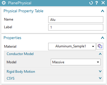
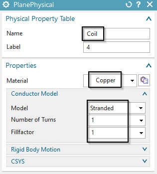
Create a tri mesh on the faces of the aluminum tube. Use the suggested mesh size value divided by 2. The system automatically creates a ’PlanePhysical’ which you can modify now.
Assign material ’Aluminum_Sample1’ from the library
’Magnetics_Materials.xml’. Name the Physical and mesh collector
’Alu’.
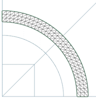
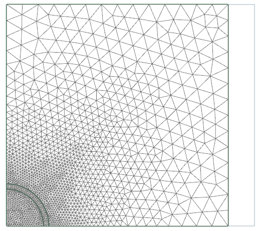
Create a tri mesh on the other faces (see picture, use suggested
element size /2) for the air. Assign a physical of type ’FluidPhysical’
and ’Air’ as material.
Hint: Do NOT mesh the coil face. This will be used later. For this part
of the tutorial the coil face stays unmeshed.
For easier post processing, click on the button ’Rename Meshes
...’ ![]() from the Magnetics toolbar. That
utility renames all meshes and therefore is a useful feature especially
with larger models and many meshes.
from the Magnetics toolbar. That
utility renames all meshes and therefore is a useful feature especially
with larger models and many meshes.
Switch to the Sim file.
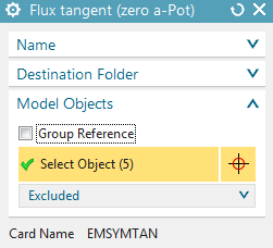
Create a first constraint of type ’Flux tangent (zero a-Pot)’ for
the symmetry at plane x=0.

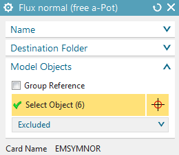
At plane Y=0 (and at the top edge) we need normal flux lines. So
create a constraint of type ’Flux normal (free a-Pot)’ on these 6
edges.
Background: These two conditions define the symmetric situation. Notice
that the normal condition could also be left, because normal flux lines
is the default behaviour of this magnetic vectorpotential formulation at
boundaries.

Define a time dependent flux density in the air.
Background: The task-description of TEAM 1a demands an exponential varying magnetic flux density with time. We create this flux density by using a given potential on the boundary edge. We use the trick that any magnetic potential difference between two positions results in magnetic flux through the area between the two positions. This constraint leads to an equally distributed flux density in a homogeneous area. Only the aluminum-tube will disturb the homogeneous flux density. And this disturbing effect shall be analysed.
Create a constraint of type ’Given a-Pot by Math-Function’ on the
right edge. Key in the displayed formula into the field ’Math Function’.
Click OK.
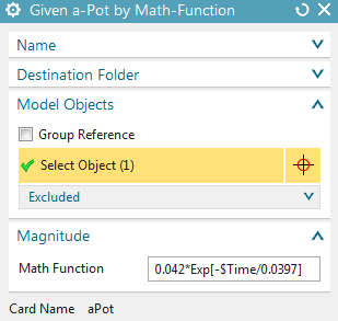

Hints: The factor 0.042 results from the requirement that at the beginning of the time period a constant flux density of 0.1 T shall exist. This value was computed by a pre analysis without aluminum-tube. The syntax for this formula and further possibilities are described in the Getdp-documentation.
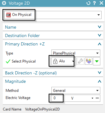
Create a zero voltage load with type ’On Physical’ on the alu
tube. This is necessary to fix the z direction degree of freedom for the
electric current in this conductor. Such a condition must always exist
on electric conductors in dynamic simulations. In case the optional
frequency solution is there, this voltage load must be created for this
solution additionally.
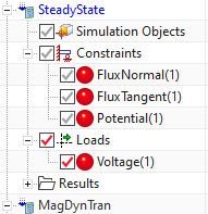
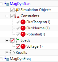
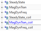
Put all constraints and the load into all solutions. The
solutions, two or three - depending on the optional frequency solution -
in the navigator should look like in the picture.
First solve the ’SteadyState’ solution. Then solve solution ’MagDynTran’ that restarts from the previous one.
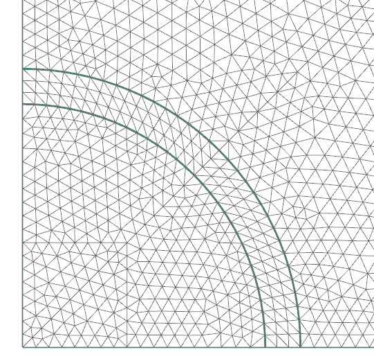
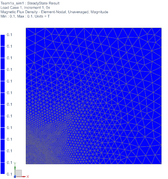
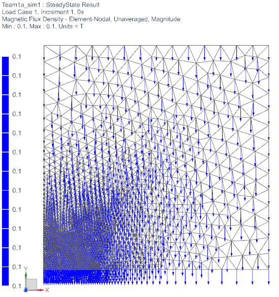
Check the SteadyState result:
Check that at the beginning of the time period flux density is
exactly 0.1 Tesla in the whole area. The directions are all
vertically.
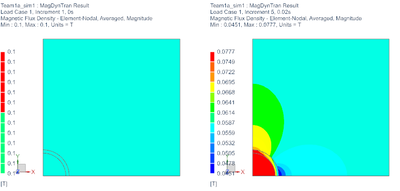
Then check the transient result:
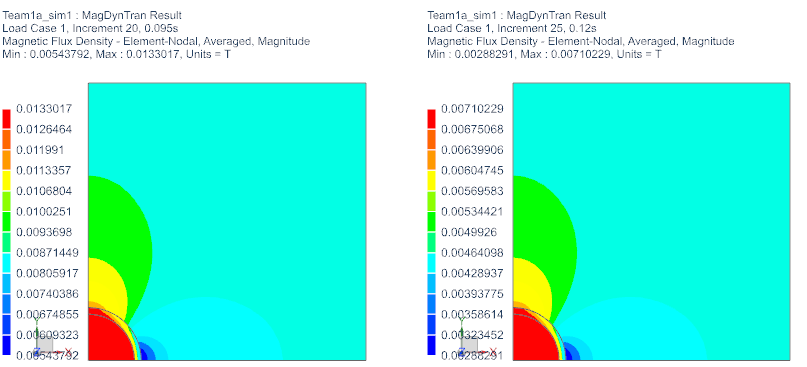
Check how magnetic flux density varies with time. The following
pictures show magnetic flux density at the beginning, in the middle and
at the end of the time period.
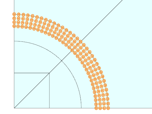
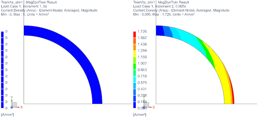
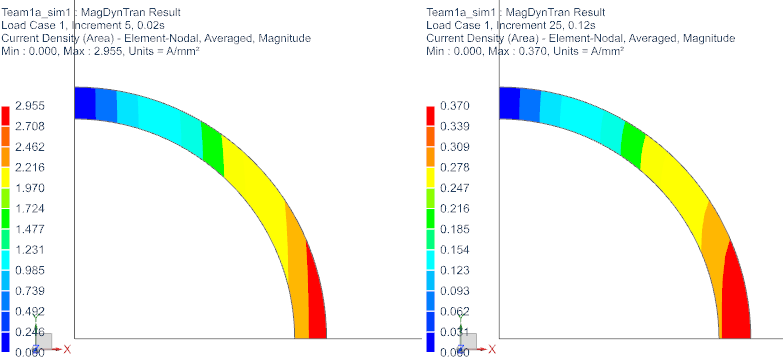
Check the induced current density in the aluminum-tube at
increments 1, 2, 5 and 25.
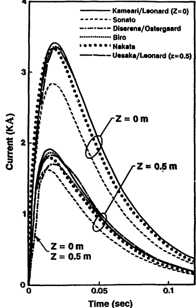
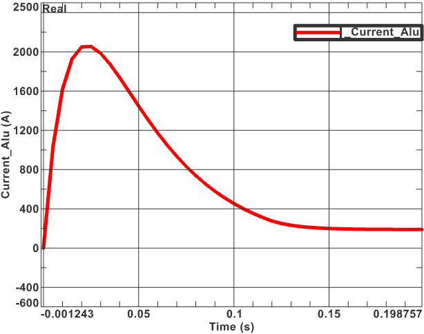
In the following picture, we see two different graphs which plot
the current in the Alu over time. The graphs in the left picture result
from several benchmark teams using different numerical codes, whereas
the right one shows the simulated solution in our code NX-Magnetics.
Since the left approaches are all centered around our simulation, we can
say that our simulation has a derivation of about 10%.
As an alternative to the first part of the example we want to realize the flux density condition now by giving a time dependent current on the right face. The resulting magnetic field leads to the same flux density.
Open the previously created Sim file.
Clone all solutions (2 or 3, in case the frequency solution is
also there). Rename the new ones with extension ’_coil’.
in the transient one, change the ’Initial Condition - Restart Solution Name’ to the new one: ’SteadyState_coil’.
Change to the Fem part and mesh the face right in the picture.
Assign material copper and stranded properties with 1 turn. Using this
stranded method you will get a homogeneous distribution of the current
over the face.

Change to the Sim file and
In all new solutions (_coil), remove the previously used potential constraint.
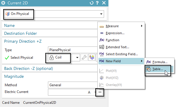
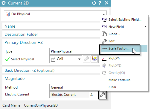
Create a load of type ’Current 2D’, with type ’On Physical’.
Accept the default method ’General’.
Select the newly created physical ’Coil’.
Click the ’equal’ button ![]() and select the table function as shown
in next picture.
and select the table function as shown
in next picture.
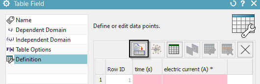
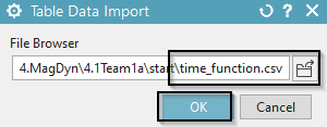
In following dialogue ’Table Field’ click 4 times ’Next’ to
accept some defaults. Then, click ’Import from File’ and select the file
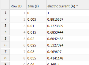
’time_function.csv’ from the ’start’ folder, that already contains data
points for the exponential function. OK.
All the points are transferred into the dialogue. Click OK.
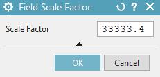
Back in the prior dialogue, insert a scale factor of 33333.4 to
the field by simply adding it to the formula as shown:
Add this new load to both solutions.
For the optional frequency solution, such a tabular definition is not possible. Instead, a fixed value current load with 1 A can be created.
Solve the two (or three) solutions in the same order as before.
Post-processing.
All results should be very near to those we have analysed in part one of
this exercise. (Blank the copper mesh in the post view to compare the
results to the first exercise.)
The tutorial is complete. Save your parts and close them.
In this tutorial we show how to create a Resonant Circuit in a 1D
Simulation. We calculate the circuit current over time and verify the
result with a analytic calculation. Later we replace the 1D resistance
with a 3D geometry. This concept can be used to connect realistic 3D
geometries with 1D circuits.
Start the program NX or Simcenter 3D.
In Simcenter, create a new file. Key in for name ’ResonantCircuit1D’ and click OK.
From toolbar Application click on ’Pre/Post’ ![]()
Click in toolbar ’Magnetics’ on ’New FEM and Simulation
(Non-Manifold)’ ![]()
Create a Solution with type ’Magnetodynamic Frequency’. In ’Output Request’, ’Plot’, activate ’Electric Potential (phi-Pot). In ’Table’, activate ’Circuit Voltage’ and ’Circuit Current’. As Frequency use 50Hz.
In ’Edit Solver Parameters’, select ’Create, keep txt Files’.
Click ’Node Create’ from toolbar ’Nodes and Elements’. Create 4 nodes, approximatly in form of a rectangle. Use any positions.
Create a ’1D Connection’ and select with ’Node to Node’ the first two nodes. Set the type to ’Resistor’. Create a second 1D Connection, select the next two nodes with type ’Inductor’. Create between the last two nodes another 1D Connection with type ’Conductor’.
Edit the physicals of the resistor. Key in \(1\Omega\) for ’Electric Resistance per Element’. Do the same for the ’Inductor’ with 1H and 1(Farad) for the ’Capacitance’ of the ’Capacitor’.
Switch to the Sim File and click ’Load Type’, ’Voltage Harmonic’. Switch to ’On Circuit’ and select the two open nodes as primary and secondary node. Key in 1V.
Solve the Solution.
Open the file with the extension ’.CurrentCircuit.txt’.

Shown is the real and imaginary part of the circuit current at every
component. Since we have a serial circuit, the current is always the
same.
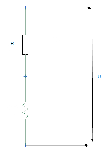
We set up a differential equation of the ’Serial Resonant Circuit’ to
calculate the current over the time t. The differential equation results
from the sum of the circuit voltages: \[U(t)
= U_{R} + U_{L} + U_{C}\] \[U(t) = R
\cdot I(t)+ L \cdot I^{'}(t) + \frac{1}{C} \cdot \int_{}^{}I(t)
dt\] We derive the equation by time to avoid the calculation with
an integral. \[U^{'}(t) = R \cdot
I^{'}(t)+ L \cdot I^{''}(t) + \frac{1}{C} \cdot
I(t)\] with \(R = 1\Omega\),
\(L = 1H\), \(C = 1F\) and \(U(t) = cos(2 \cdot \pi \cdot 50Hz \cdot
t)\), so \(U^{'}(t) = 100\pi \cdot
cos(100\pi \cdot t)\).
We use the following mathematical approach: \[I_{p}(t) = D_{0} \cdot sin(bt) + E_{0} \cdot
cos(bt)\] That approach and it’s derivations are inserted into
the differential equation and after some simplifcations we get:
\(cos(b \cdot t) \cdot b + (sin(b \cdot t)
\cdot 0) = cos(b t) \cdot (D_{0} \cdot b - E_{0} \cdot b^{2} + E_{0}) +
sin(bt)\cdot(-E_{0} \cdot b - D_{0} \cdot b^{2} + D_{0})\)
with \(b = 100\pi\) and a coefficient
comparision two equations with two variables result.
Solving the equation system gives \[D_{0} =
1.013 \cdot 10^{-5}, E_{0} = -3.18 \cdot 10^{-3}\] We lead this
back to our approach and get a equation describing two oscillations:
\[I(t) = 1.013 \cdot 10^{-5} \cdot
sin(100\pi \cdot t) - (-3.18 \cdot 10^{-3}) \cdot cos(100\pi \cdot
t)\]
The sum of the two oscillations finally results in \[I(t) = 3.18A \cdot 10^{-3} \cdot sin(100\pi \cdot
t - 1.571)\] Converting this into a complex number gives \(I = 1.013 \cdot 10^{-5} -j3.18 \cdot
10^{-3}\). This is the settled result for the current behavior
over time and matches precisely with the result of the simulation.
We now replace the 1D Resistor with a 3D geometry. Because of the
material properties and the geometry, there arises a resistance.
Following we open an existing model and walk through some interesting
features.
Download the model for this tutorial from the following
link:
https://www.magnetics.de/downloads/Tutorials/4.MagDyn/4.8ResonantCircuit.zip
Extract the zip-archive. In Simcenter, click Open ![]() and
navigate to the folder of the extracted archive. Select the file
’ResonantCircuit3D_sim1.sim’ and click OK.
and
navigate to the folder of the extracted archive. Select the file
’ResonantCircuit3D_sim1.sim’ and click OK.
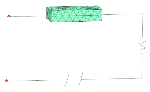
The meshes for the air and the resistor are already created. We use a self made material for the resistor and get a resistance of \(1.07\Omega\) which nearly corresponds to the prior 1D simulation.(\(1.0\Omega\))
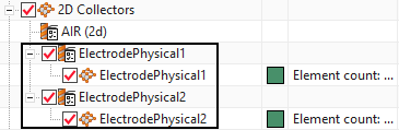
There are two 2D meshes of type ’ElectrodePhysical’. These are
necessary to connect a 1D connection to a 3D geometry. They don’t
contain any physical properties.
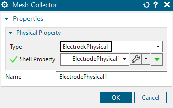
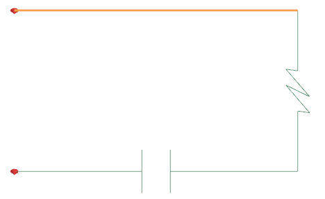
To finally connect the 2D electrode with the outside circuit we
need a 1D connection of type ’Connector’. Such a connector must be
between a node of the electrode and another node in the circuit. See
picture below.
Switch to the Sim File and solve the solution.
Open the file with the extension ’.CircuitCurrent.txt’

Shown is the circuit current, which matches well with the 1D simulation. The small deviation results from the slight difference in the ohm resistance.
The tutorial is finished.
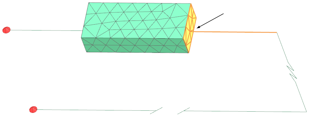
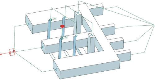
In this example there is a network defined connecting different
electrodes of several conductors. The conductors are of 3D, 2D and 1D
type. The example shows how to set up these features. A harmonic current
load is applied on the left and right points of the network (see
picture). So the electric current flows through all conductors.
Download the model files for this tutorial from the following
link:
https://www.magnetics.de/downloads/Tutorials/4.MagDyn/4.5Network.zip
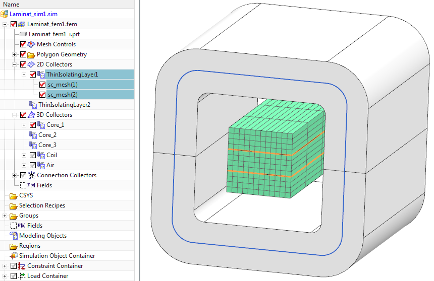
In this example there is a core in a coil running in a magnetodynamic
simulation. The core has two isolating layers which avoid eddy currents
to cross those layers. The example shows how to set up these
features.
Download the model files for this tutorial from the following
link:
https://www.magnetics.de/downloads/Tutorials/4.MagDyn/4.6Laminate.zip
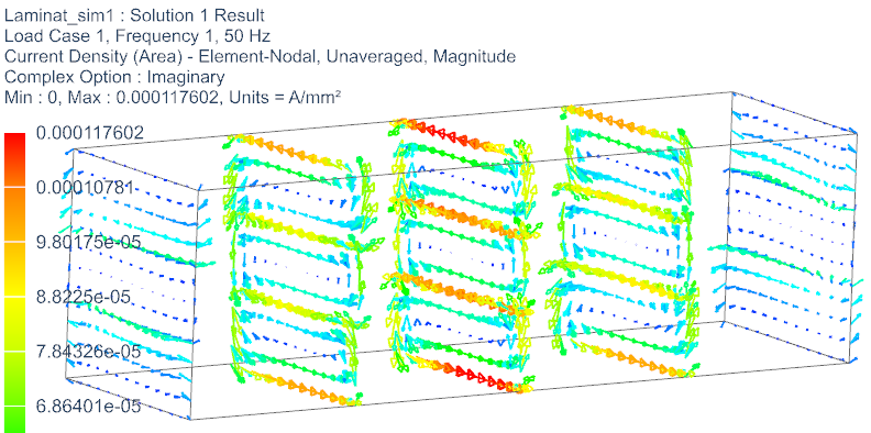
The following figure shows the meshed core and the coil. Two orange
sheets (highlighted) are the isolating layers. These are meshed in 2D
and assigned to a physical of type IsolatingLayer.
Next figure demonstrates the eddy currents in the core and how they are
hindered from crossing the isolating layers.