Electrokinetic

Circular Plate

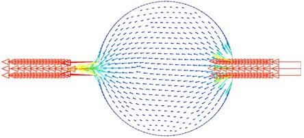
Goal of this analysis is to analyze the electric current flow in a circular plate to compute its ohm resistance.
Download the model files for this tutorial from the following link:
https://www.magnetics.de/downloads/Tutorials/2.EleKin/2.1CircularPlate.zip
This model already contains all needed properties and parameters.

Preparation

1. Unzip the archive. There will be one folder ’start’ and one ’complete’.

2. Start the Program Simcenter (or NX).

3. In Simcenter, click Open and navigate to folder ’complete’. Select the file ’CircularPlate_sim1.sim’ and click OK. (Maybe you must set the file filter to ’sim’)

4. Click from toolbar ’Application’, ’Pre/Post’.

Sim File Check

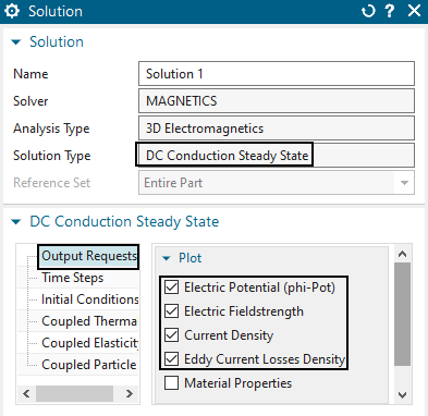
1. Edit the already existing Solution ’Solution1’, to check the properties.

   • The ’Analysis Type’ is ’3D Electromagnetics’, the ’Solution Type’ is set to ’DC Conduction Steady State’.
     Hint: This solution type simulates the electric field in electric conductors and the resulting electric current. The magnetic field is not considered. From the electric current, the geometry and the boundary conditions, the ohm resistance can be derived.

   • Under ’Output Requests’ ’Plot’, ’Electric Potential (phi-Pot)’, ’Electric Fieldstrenght’, ’Current Density’ and ’Eddy Current Losses Density’ are active to check these results.

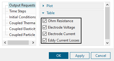
   • In ’Table’, ’Ohm Resistance’ and some others are active.
     

2. The ’Result Graphs (afu)’ in ’Edit Solver Parameters’ is set to ’Create, keep txt Files’.

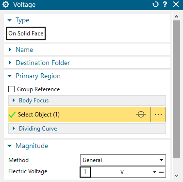
3. Edit the load ’Voltage(1)’. The type is ’On Solid Face’ and the face of the supply line is selected. The ’Electric Voltage’ is set to 0V.

4. Edit the second load. The other side of the supply line is selected and the ’Electrode Voltage’ is set to 1V.
   

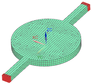
5. Make the Fem File to the displayed part.

6. In ’3D Collectors’, edit the mesh collector ’Copper’. Edit the physical and verify the material is set to copper.

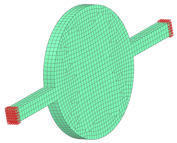
7. Check the properties of the 3d mesh. In this case there is a hex mesh used. The use of tet mesh is also possible.

8. Solve the Solution

Post Processing

1. Open the File with the extension ’.Resistance.txt’.
   The calculated resistance of the full geometry circuit plate is shown.
   

Result Comparison with Analytic

For analytic calculation, we use a substitute resistance to calculate the ohm resistance of the circular plate. \[R_0 = \frac{2a}{2bd\kappa} = \frac{0.2m}{2 \cdot 10mm \cdot 20mm \cdot 58S/m} = 8.6207 \cdot10^{-6}\Omega\] with \(a = 100mm\), \(b = 10mm\), \(d = 20mm\), \(\kappa = 58 S/m\)


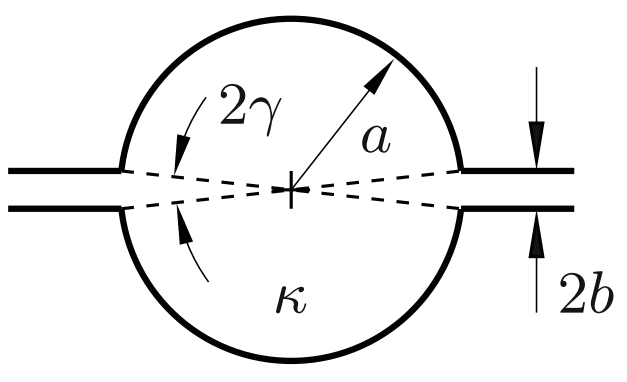
Next we have to determine the resistance of the circular plate depended on the entrance angle \(\gamma\). \[\gamma = sin^{-1} \cdot (\frac{a}{b}) = 0.10016 [rad]\]
The ratio between the resistance of the circular plate \(R\) and \(R_{0}\) is: \[\frac{R}{R_{0}} = \frac{2\gamma}{\pi} \cdot (1-ln(\frac{\gamma}{2})) = 0.2543\]
So, the resistance of the plate \(R\) is: \[R = \frac{2\gamma}{\pi} \cdot (1-ln(\frac{\gamma}{2})) \cdot R_{0} = 0.2543 \cdot 8.6207 \cdot 10^{-6}\Omega = 2.193 \cdot 10^{-6}\Omega\]
The resistance for the supply line is calculated by: \[R_{sup} = \frac{a}{2bd \kappa} = \frac{0.2m}{2 \cdot 10mm \cdot 20mm \cdot 58S/m} = 4.3103 \cdot 10^{-6}\Omega\]
The combined resistance is:
\(2 \cdot R_{sup} + R = 2 \cdot 4.3103 \cdot 10^{-6}\Omega + 2.193 \cdot 10^{-6}\Omega = 1.081 \cdot 10^{-5}\Omega\)

Source: Manfred Filtz, Heino Henke. Übungsbuch Elektromagnetischer Felder. Berlin: Springer Berlin Heidelberg, 2007

• Simulation Result: \(1.066 \cdot 10^{-5}\Omega\)

• Analytic Result: \(1.081 \cdot 10^{-5}\Omega\)

• Deviation: 1.4%