Magnetostatic

Magnetostatics is used when information of the magnetic field that surrounds a conductor is needed. In this context, a DC Conduction Steady Steate analysis is sometimes used as a preprocessing step, and the resulting currents are used as input to a subsequent magnetostatics analysis. This would be the case, for example, when analysing electromagnets. The fundamental material property for performing magnetostatics analysis’ is the relative magnetic permeability \(\mu_{r}\). For nonlinear magnetostatics analyses, a more general material relationship may be needed, such as a functional relationship between the magnetic field and the magnetic flux density: a so-called B-H curve. The ultimate goal of a magnetostatics analysis is, in many cases, to compute the forces and torques in a system of magnetic components.

Analysis of permanent magnets constitutes an important, special case of magnetostatics analysis. In this case, a permanent magnetization is the source of the magnetic field instead of an electrical current. In such cases, the magnetic flux strength and direction as well as forces are important analysis results.

Core and Inductor (Beginner)

In this example it is shown how to build up and analyse simple models in 2D or axial-symmetric situations. An electric coil is positioned near a magnetic core. The electric current in the coil creates a rotating magnetic field (ampere law), that affects the magnetic core material. We want to calculate for the magnetic field strength and flux density in the core. Also, we want to find the mechanical forces acting on the core.
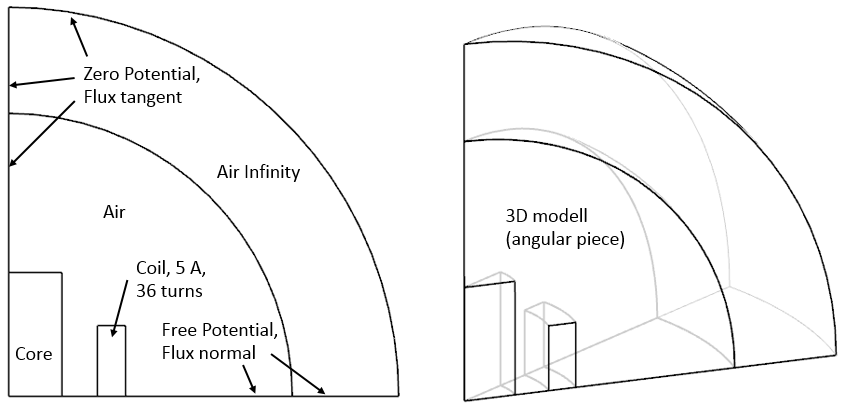
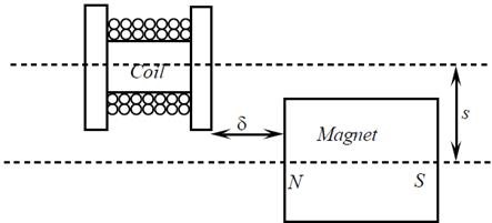
The picture below left shows a sketch representing the model. In the 2D case, we assume an extruded geometry that is simulated by flat 2D elements and an applied thickness (150 mm.) On the right side, there is shown how this would look like in an axial-symmetric case (an angular piece is shown).
The coil is loaded with electric current of 5 Ampere DC and 36 winding-turns.
Following to this 2D analysis (with thickness) we will use the same model to analyse for the axial-symmetric situation.

Estimated time: 45 min. Follow the steps in Simcenter:

Preparations

1. download the model files for this tutorial from the following link:
   https://www.magnetics.de/downloads/Tutorials/3.MagSta/3.1CoreInductor.zip

2. unzip the archive. There will be one folder ’start’ and one ’complete’.

3. Start the Program Simcenter (or NX). Use Version 10 or higher.

4. In Simcenter, click Open and navigate to folder ’start’. Select the file ’CoreInductor.prt’ and click OK. (Maybe you must set the file filter to ’prt’)

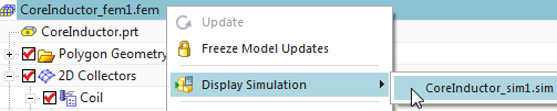
5. From toolbar Application click on ’Pre/Post’ and the system switches into the simulation application.

6. Hints: All information describing the Simcenter simulation is managed in basically three files (picture below): The Sim, the Fem and the Idealized file. The Sim file contains the solution, boundary conditions, loads. The Fem file contains the finite-element meshes, material properties and other physical properties. The Idealized file is optionally and can be used for simplifications or modifications of the CAD geometry without changing the original CAD file.
   

Fem and Sim File Creation

Following, we will first create the Fem and Sim file structure and then we will fill it up with data. We will create the Fem and Sim files in two separate steps, which has the advantage that we can choose a Fem-file-template. The template already contains basic material properties. The ’Simulation Navigator’ will allow us navigating in the file-structure.

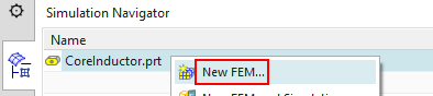
1. Click on ’New FEM’ .
   (’New FEM’ is also found at RMB on the master part in Simulation-Navigator)
   

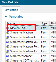
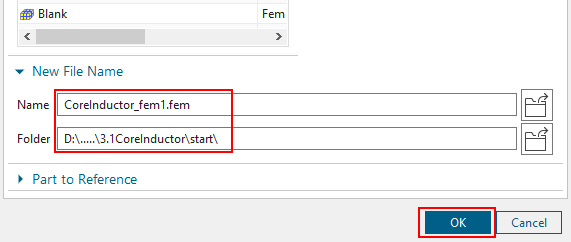
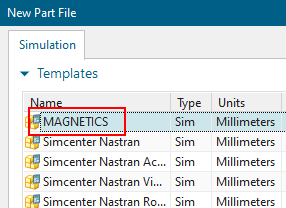
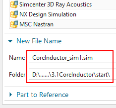
2. In window ’New Part File’, select the MAGNETICS-template, check file name and folder (use work part location for all parts) and click ’OK’.
   
   (Messages ’Unsecure Solver Language File’ may appear and can be accepted)

3. The window ’New FEM’ appears.
   

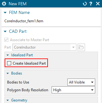
   • Switch off ’Create Idealized Part’ because the geometry is already very simple. Thus, we will have one file less and the file structures is simpler.

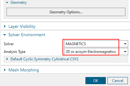
   • Set the Solver to MAGNETICS and Analysis Type ’2D or axisym Electromagnetics’ and click OK. The Fem file is created.

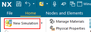
4. Click on ’New Simulation’ (or find this RMB on the Fem file).
   

5. A window ’New Part File’ appears in which you again select the MAGNETICS-template and check for the new name and folder. Click ’OK’. In a further window ’New Simulation’, also click ’OK’.
   
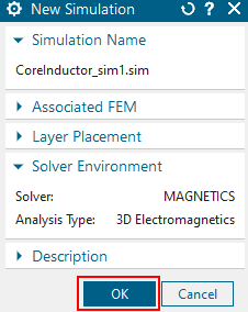
   The Sim file is now also created.

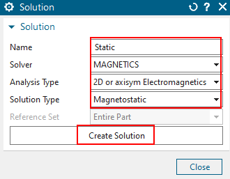
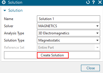
6. Following, a window ’Solution’ appears
   (if this does not automatically appear, click on ’Create Solution’) )

   • assign the Name ’Static’, accept the default Solution Type ’Magnetostatic’.
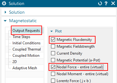
     Click ’Create Solution’ and

   • in register ’Output Requests’, activate the results ’Magnetic Fluxdensity’ and ’Nodal Force - entire (virtual)’.
     

   • Click on register ’2D’ and set the ’Thickness’ to 150 mm.
     

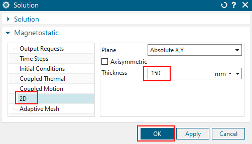
   • All other settings are well predefined. Click OK. The solution will be created and the system will jump to the Fem file.

Fem File Steps

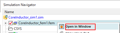
1. We are now going to create finite element meshes. Therefore, use the Simulation Navigator to set the Fem file to ’Open in Window’.
   

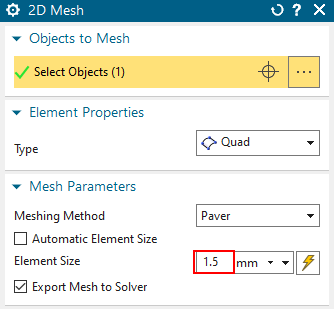
2. Mesh the Coil

   • Click on ’2D Mesh’ from toolbar Home\(\rightarrow\)Mesh and select the the coil face.

   • Set the Type to ’Quad’ and the element size to 1.5 mm.
     Hint: Tri elements or other sizes would also work.

   • Click OK and the mesh is created.
     

3. Assign Properties to the Coil

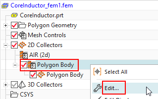
   • Double click on the newly created 2D Collector.

   • In the following window, set the Name to ’Coil’ and click ’Edit’ .
     Hint: It is recommended to assign meaningful names because those names will appear in the results and legends of all following result tables.
     

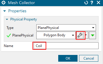
   • A new window ’PlanePhysical’ appears.
     

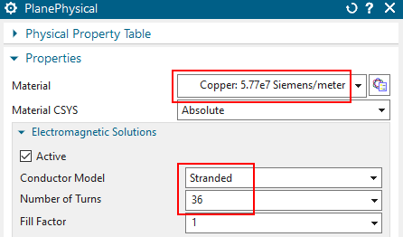
   • At ’Material’, choose ’Copper...’, from the list.
     Hint: Because we have used the Fem file template, there are already some basic materials in the list. For more flexibility, choose from many materials from libraries or define your individual material properties by clicking ’Choose Material’

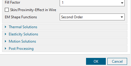
   • set the ’Conductor Model’ to ’Stranded’ and apply the value 36 for ’Number of Turns’. Accept the default 1 for ’Fillfactor’.
     Hint: The coil fill factor represents the fraction of the coil cross section that the conductor occupies. You can use this factor to adjust coil resistance.

   • Click OK, OK to finish the definition of the coil.

4. Mesh the core:

   • Click on ’2D Mesh’ and select the core face.

   • Use quad elements of 1.5 mm size. Click OK and the mesh is created.
     

5. Assign Properties to the Core

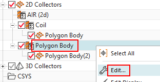
   • Double click (or RMB Edit) the newly created 2D Collector. Set the Name to ’Core’ and click ’Edit’ . The window ’PlanePhysical’ appears.
     

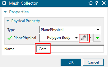
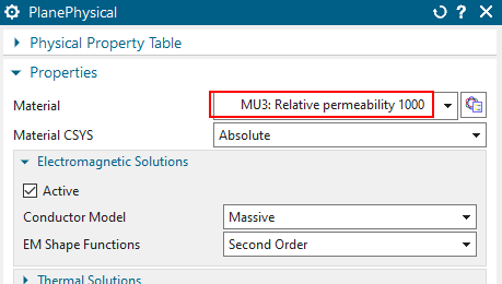
   • In the ’PlanePhysical’ window (below), select from the material list ’MU3...’, a magnetic material with relative magnetic permeability value of 1000.

   • accept the default Conductor Model ’Massive’.

   • Hint: You can use the ’Manage Materials’ feature to verify the ’relative Permeability (mur)’ of this material is correctly set to 1000.
     

   • Click OK, OK, to finish the definition of the core.

6. Mesh the inner air
   Hint: In most cases air meshes are created as the last meshing step.

   • Click on ’2D Mesh’ and select the inner air face.

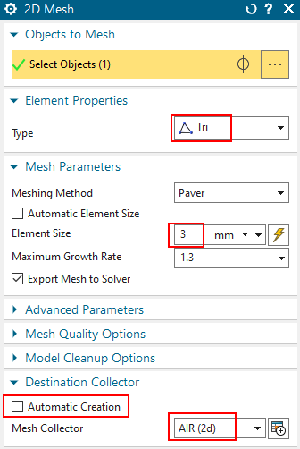
   • Set the element type to ’Tri’ and the ’Element Size’ to 3 mm.

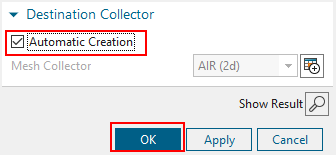
   • At ’Destination Collector’, clear ’Automatic Creation’ and verify that the ’Mesh Collector’ is set to ’AIR (2d)’.
     Hint: This collector is ready to use and comes from the Fem template.

   • Click OK and the mesh is created using the correct collector and material.
     

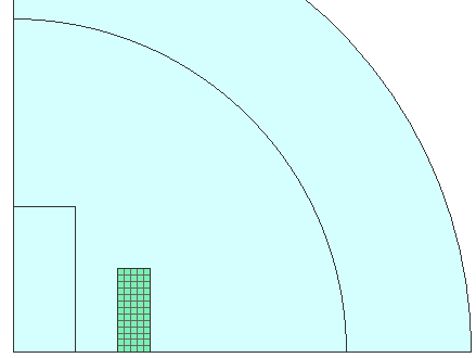
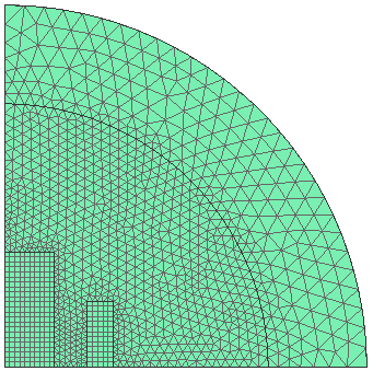
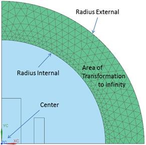
7. Meshing the Infinity Air:

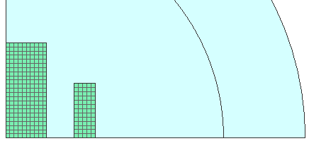
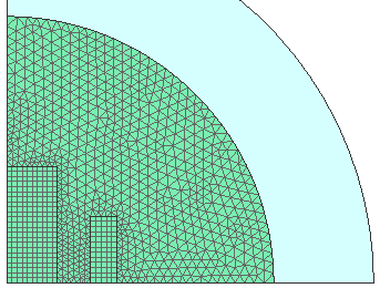
   • Background: The air around the core and the inductor geometry must be meshed to realistically model the magnetic (and in other cases the electric) field around these parts. This air geometry must be large enough to model the field. If it is too small, the simulation will model this field too "compressed" and the results may be inaccurate. To decide on the magnitude of this air geometry, one should also consider whether the field “wants” to leave the core and inductor geometry (flux leakage): if there is a closed iron path holding the magnetic flux, we would expect a small leakage and a large ball would not be necessary there. In our example, there is no such closed iron path and therefore we expect more leakage flux and the air geometry must be larger. Instead of a big-air geometry, there is also the option of using infinity elements. These infinity elements are to be used in our example. We used circular geometry, but other shapes like blocks would work as well. The advantage of a circular geometry is that this form is, so to speak, natural for the field lines. This also makes it easy to use Infinity elements.

   • Click on ’2D Mesh’ and select the outer air face.

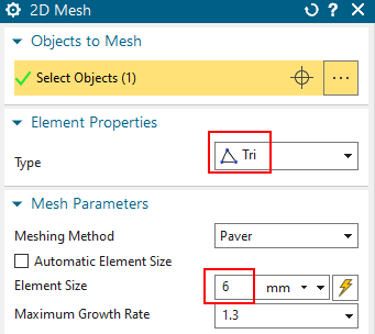
   • Use Tri elements of 6 mm size.

   • At ’Destination Collector’, activate again ’Automatic Creation’.

   • Click OK and the mesh is created.
     
     

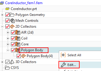
8. Assign Properties to the Infinity Air

   • Double click on (or RMB Edit) the newly created mesh collector.

   • Set the Type to ’Infinity2D’ and the Name to ’Air_Inf’

   • Click on ’Create Physical’. A new window appears.
     

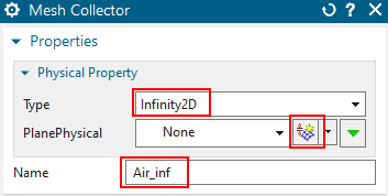
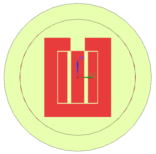
   • in the window ’Infinity2D’, key in the value 80 mm for ’Inner Radius at Shell’ and 30 mm for ’Shell Thickness’. as shown in the picture. The dimensions must correspond to the size of the infinity air layer (see picture below).
     
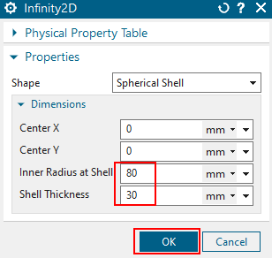
     Click OK, OK to create the Physical.

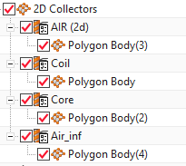
9. As the final step in the Fem file, click on the button ’Auto Rename’ from the Magnetics toolbar. That utility renames all meshes and Physicals depending on the collector-names. It is a useful feature, especially with larger models and many meshes. Post processing becomes easier, thus we recommend this always to run after the meshing is done.
   
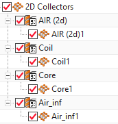
   The picture above left side shows prior, right after the auto-rename.

Sim File Steps

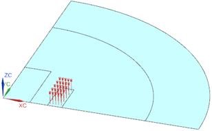
1. We are now going to create boundary conditions. Therefore, set the Sim file to the displayed part. (The meshes are blanked here for easier visibility)
   

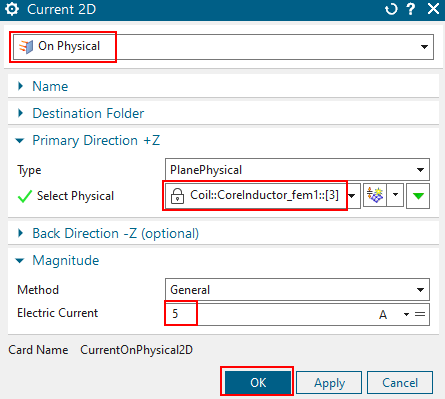
2. Create a load for the electric current on the coil:

   • Click on ’Current 2D’ from toolbar Home\(\rightarrow\)Loads and Conditions\(\rightarrow\)Load Type.

   • Accept the default Type ’On Physical’.

   • At ’Primary Direction +’, ’Select Physical’, select the Coil Physical from the list.

   • Assign the value 5 A for ’Electric Current’.

   • Click OK and the load is created.
     

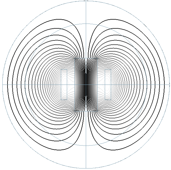
3. Understanding constraints

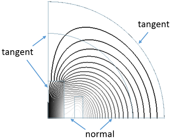
   • The model we use represents a quarter of the full model. Therefore, we must correctly apply constraints at all borders. The picture below left shows how magnetic field lines would appear in the case of a full model.

   • This allows understanding how constraints must be set in our quarter model: We need tangent magnetic field conditions at the circular border and at the vertical symmetry edges. And we need normal field conditions at the horizontal symmetry edges.

   • Such field lines can also be shown in the results of the simulation: In ’Output Requests’ activate ’Magnetic Potential (a-Pot)’ and display this result in the post processor using the iso-lines option.
     

4. Creating constraints.
   According to such needs, now we will create two tangent and one normal constraint.

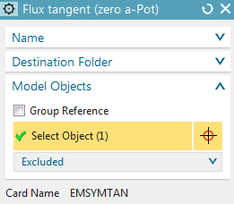
   • Click on ’Flux Tangent (zero a-Pot)’ from ’Constraint Type’. Select the outside circular edge and click OK.

   • Hint: This constraint type must always be applied at the outside air border to keep the field from leaving the computation area.
     

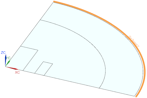
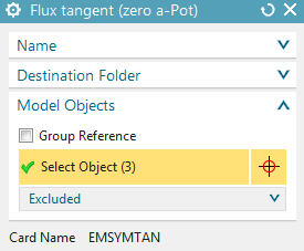
   • Again click on ’Flux Tangent (zero a-Pot)’ and select the three x=0 symmetry edges. Click OK.

   • Hint: Viewing the resulting magnetic field lines helps understanding the symmetry condition.
     

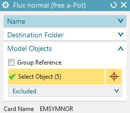
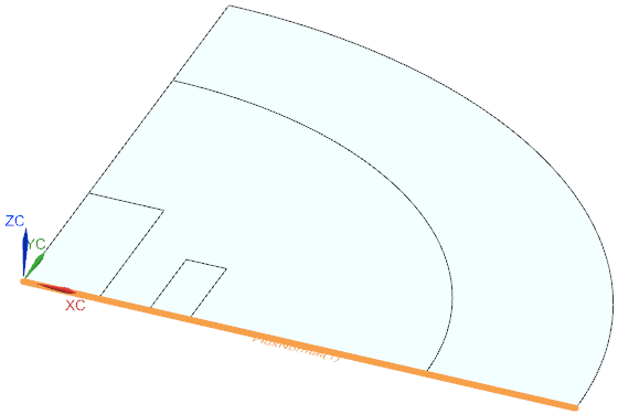
   • Click on ’Flux normal (free a-Pot)’ and select the five y=0 symmetry edges. Click OK to create the condition.
     

5. Solve the solution:

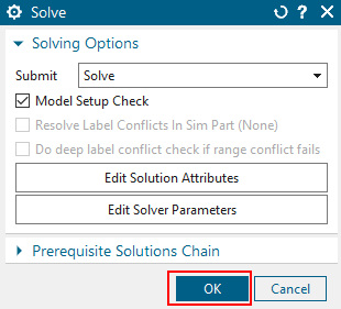
   • Click on ’Solve’ from toolbar ’Solution’.

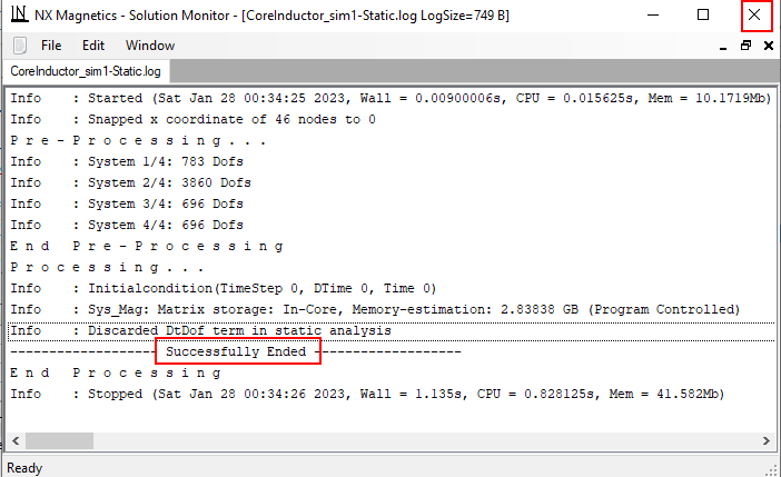
   • click OK. The solve job starts and a new window appears to monitor the solution progress. The solve job takes only a view seconds for this small model.

   • If the solution monitor shows ’Successfully Ended’, the job has ended and there should be results. Cancel the solution monitor and also other info windows that may have appeared.
     

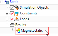
6. Post Processing Force Results

   • Double click on the ’Result’ node in the Simulation Navigator.
     Hints: The system opens the result file and switches to the post processor. The field results are managed using the ’PostProcessing Navigator’ (see below right).
     

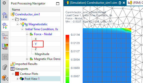
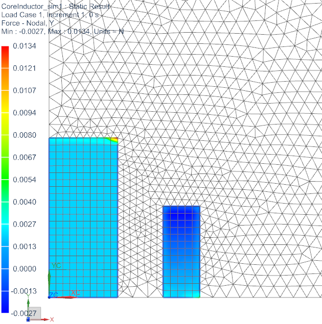
   • Double click on ’Force - Nodal Y’ to plot the force distribution in Y direction. There appears a PostView showing this.

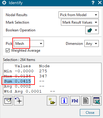
   • Click on ’Identify Results’ from toolbar ’Results’

   • set ’Nodal Results’ to ’Pick from Model’ and option ’Pick’ to ’Mesh’ and select the face of the core.

   • The sum of all values on the core is evaluated and written into the ’Identify’ window. This resulting force sum is about 0.04 N.
     Hints: The defined thickness value of 150 mm is already taken into account.
     

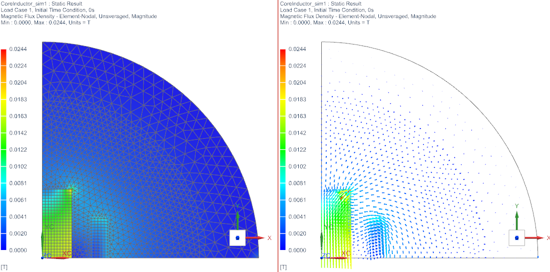
7. Post Processing Magnetic Flux Density

   • To plot the distribution of magnetic flux density double click on ’Fluxdensity - Element Nodal Magnitude’.

   • to display the magnetic flux density by arrows, switch from ’Contour’ to ’Arrows’ in toolbar ’Results’. These vectors show the direction of the field lines.
     

Axisymmetric Analysis of Core and Conductor

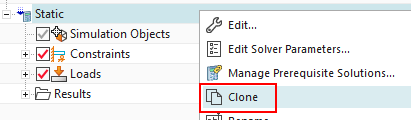
To analyze in an axial symmetric way (axis is Y) using the same geometry follow these steps:

1. Clone the solution and

2. Rename the new solution to ’Axisym1’.
   

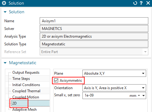
3. Choose ’Edit Solution’ on the new ’Axisym1’ and switch to register ’2D’. Activate ’Axisymmetric’ and click OK.
   Hint: To use axis symmetric analysis, it is necessary to place all elements on the x/y plane for positive x. The axis must be Y.
   

4. Solve the solution and post process the results:

5. Check the force sum in Y direction again. It should be about 0.08 N. The axisymmetric effect (2*Pi) is already taken into account.

6. The tutorial is complete. Save your files and close them.

Static Force on Solenoid (TEAM 20) (Beginner)

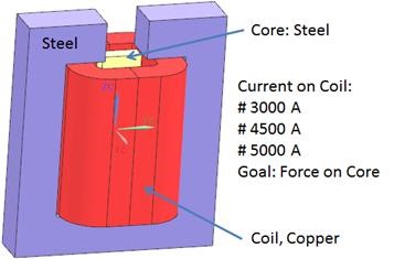
This example is a convenient training for all those who want to do electromagnetic analysis with complex 3D geometries, because it contains most necessary skills for dealing with this.

The Team20 benchmark is a test example for electromagnetic analysis software tools. There are measured force-results available that we will use for comparison with the simulation-results. We will use a nonlinear B-H curve that includes saturation effects for the core and iron parts.

For meshing, we want to exploit the ’Non-Manifold’ strategy, which automatically finds adjacent face pairs and creates conformal meshes (e.g. coincident nodes) at those interfaces. Thus, no Mesh-Mating conditions are needed any more. Unfortunately, this must be done differently in the different NX/Simcenter versions. Prior to NX 1953 (2021.1) this approach is not possible at all and must be replaced by the conventional Mesh-Mating method.

Necessary time: 1 h.

Preparations

1. download the model files for this tutorial from the following link:
   https://www.magnetics.de/downloads/Tutorials/3.MagSta/3.2Team20.zip

2. unzip the archive. There will be one folder ’start’ and one ’complete’.

3. Start the Program NX or Simcenter . Use Version 12 or higher.

4. In NX/Simcenter, click Open and navigate to folder ’start’. Select the file ’Team20.prt’ and click OK. (Maybe you must set the file filter to ’prt’)

5. From toolbar ’Application’, click on ’Pre/Post’ .
   The system switches into the simulation application.

6. Hint 1: All information describing the simulation is managed in basically three files (see below): The Sim, the Fem and the Idealized file. The Sim file contains the solution, boundary conditions, loads. The Fem file contains the meshes, material properties and other physical properties. The Idealized file is optionally and can be used for simplifications or modifications of the geometry without changing the original CAD file.
   
   Following, we will first create this file structure and then we will fill it up. The ’Simulation Navigator’ will allow us navigating through the structure.

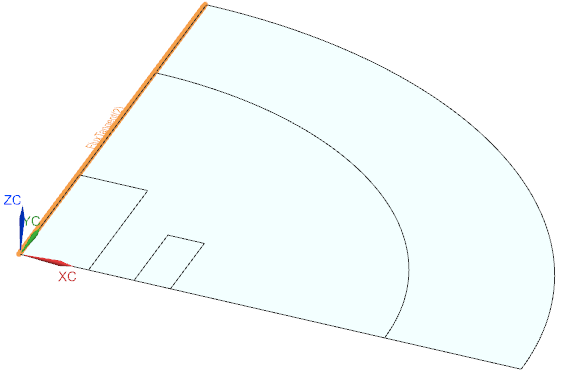
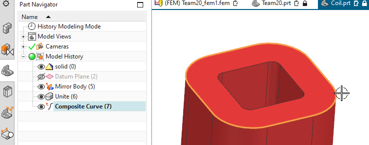
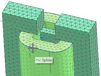
7. Hint 2: Notice, in the CAD Model, there is a spline curve extracted from the outside edges of the coil (see highlighted in below picture). This spline will be used to define the winding directions. It is necessary, that this spline is one single curve. In case there are multiple curve segments, there must be done a ’Join Curve’ operation to make one spline out of them. We will later have to activate one special button to transfer this spline into the Fem file.
   

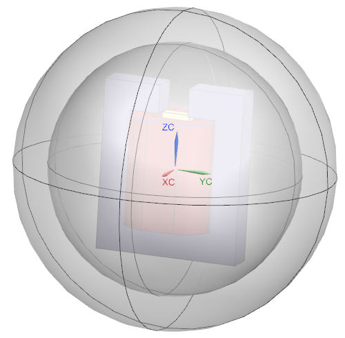
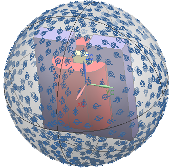
8. Hint 3: A spherical air volume is placed around the solid geometry and an additional spherical shell is placed around the sphere. This sphere is necessary to model the magnetic (and in other cases also the electric) field in air. The shell additionally models the infinity air. We could solve without the infinity air, but in that case the air volume would have to be large enough to model the field. In case it would be too small, the simulation would model that field too much ‘compressed’ and results would become inaccurate. To decide about the size of such an air volume, it should also be considered whether the field ‘wants’ to leave the solid geometry (flux leakage): If there is a closed iron path, holding the magnetic flux like in our case, there is no need for a big sphere. In other cases, there may appear more flux leakage and the air volume should be larger. Instead of using a large air volume, we rather want to use infinity elements just like we already did in the previous tutorial ‘Core and Inductor’. In this example, we use a sphere, but alternatively box geometries would work as well. Advantage of a sphere is that it is kind of natural for the field lines. Also this makes it simple using infinity elements.
   

Create Fem and Sim Files

This step must be done differently in the different NX/Simcenter versions because of the non-manifold feature we want to use. For more details, see chapter ’Recommended System Settings’.

1. Version 2212: In toolbar Magnetics, click ’New Fem and Sim (Non Manifold)’. This runs a script to create the Fem and Sim files from templates with non-manifold feature.
   

2. Version 2007 (2022.1) and 2206 (2022.2):

   • Activate the customer default ’Create Non-manifold Polygon Bodies’.

   • Create a ’New FEM’, select the MAGNETICS template.

   • Create a ’New Simulation’, also select the template.

   • The creation of the solution continues below.

3. Version 1953:

   • Activate the early access feature ’Allow updates related to Electro Magnetics’.

   • Create a ’New FEM’, select the MAGNETICS template.

   • Create a ’New Simulation’, also select the template.

   • The creation of the solution continues below.

Create the Solution

1. In toolbar ’Home’, click on ’Create Solution’

2. Accept the Solver ’MAGNETICS’ and the Analysis Type ’3D Electromagnetics’,

3. Accept the default Solution Type ’Magnetostatic’.

4. Click ’Create Solution’.

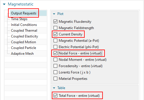
5. In register ’Output Requests’, ’Table’, activate ’Total Force - entire (virtual)’ to enable the system calculate forces by the virtual energy method.

6. to see these forces in the plots and also the applied currents, also activate in ’Plot’ ’Current Density’ and ’Nodal Forces - entire (virtual)’.
   

7. Click OK to finish the Solution window.

Parametric Meshing

Following, we will create all element-sizes using one control-parameter ’MeshFactor’. This makes it simple later to do studies with different mesh-sizes and therefore, we recommend this approach.

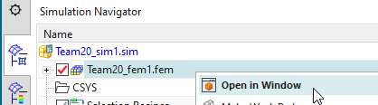
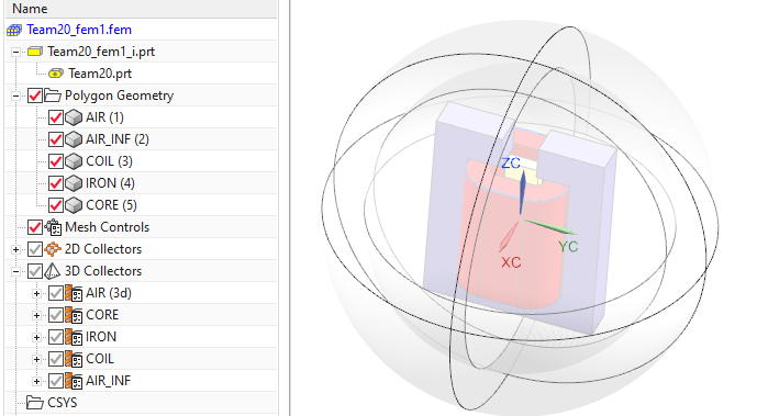
1. Do a ’Open in Window’ to the Fem part.
   

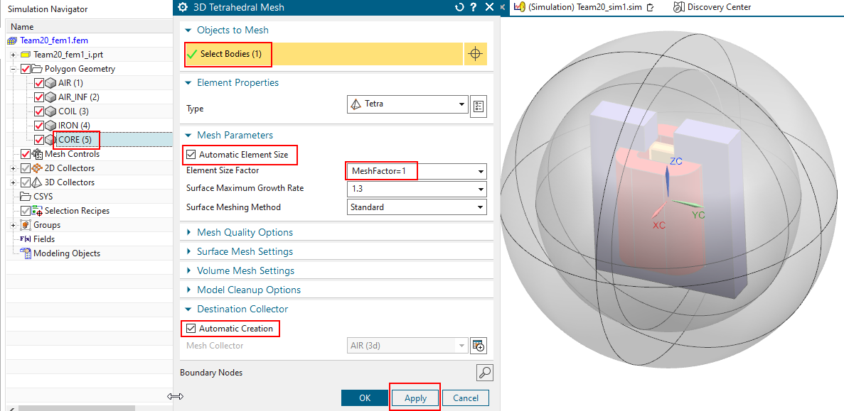
2. Mesh the CORE: Start the mesher ’3D Tetrahedral’ , select the core body (either in the graphics window or in the Polygon Geometry list) and activate ’Automatic Element Size’. In the field ’Element Size’, key in ’MeshFactor=1’ to create and initialize the parametric expression. Check, that ’Destination Collector’ is ’Automatically Creation’ and click ’Apply’. The mesh is created.
   

3. Mesh the remaining parts with nearly the same settings as follows:

   • Select the IRON body, click ’Apply’.

   • Select the COIL body, click ’Apply’.

   • Select the AIR body, set ’Mesh Collector’ to ’AIR (3d)’, click ’Apply’.

   • Select the AIR_INF body, click ’Apply’.

   Hint: the order of creation of meshes is quite important: Following meshes must always connect to the existing nodes of prior meshes. Thus, we should always start with the most important parts.

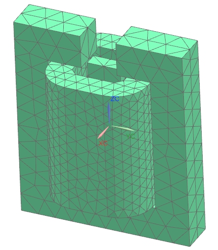
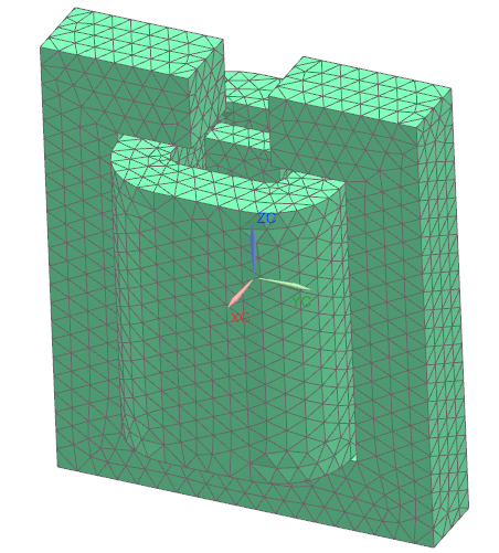
4. The meshes are still quite coarse, because of the MeshFactor=1. We want to globally reduce the mesh size to the half. Thus, change the expression ’MeshFactor’ to 0.5. This is done in the ’Expressions’ window (Menu, Tools, Utilities, Expressions).
   
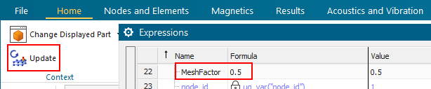
   After the new value is set, click the ’Update’ button and all elements will become smaller. The picture below shows left the old and right the new meshes of core, iron and coil.
   

Define Core/Iron Material with Nonlinear B-H Curve

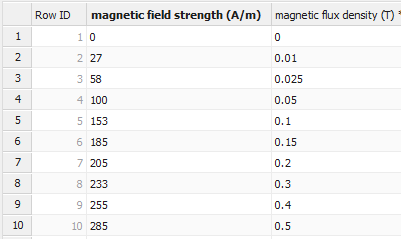
In this chapter, we define a typical steel material that is used for the core and iron bodies. This material shows a nonlinear relationship between magnetic flux-density (B) and magnetic field-strength (H). Such a relation is often the case for steel and iron. Many material properties are already available in the material library, but often, we must insert individual data and define a individual material. The data points with H-B pairs are stored in a csv file (Team20MaterialCurve.csv) in the ’start’ folder of this tutorial. Proceed as follows to create a new material with these:

• Click ’Manage Materials’ and ’Create Material’ at the bottom right.

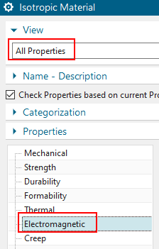
• Set ’View’ to ’All Properties’ and select the register ’Electromagnetics’. Key in a name, for instance ’Team20 Material’. Set the ’Model’ to ’Low Frequency’ (see below).
  

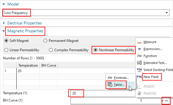
• Scroll down and set ’Magnetic Properties’ to ’Nonlinear Permeability’ (above right). Key in a ’Temperature’ of 20 degrees Celsius.

• Right to field ’BH Curve’, select the ’\(=\)’ and choose ’New Field’ and click ’Table’.

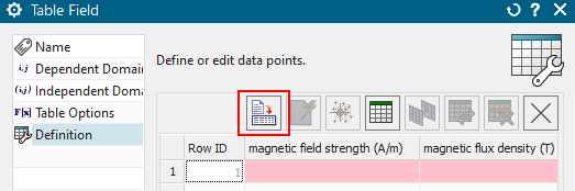
• In the next window, select ’Import from Text File’ and scroll to the ’start’ folder of this tutorial. Select the file ’Team20MaterialCurve.csv’ and click OK. The picture below right shows the ’Table Field’ window with the new data.
  

• Click OK, Close. The material is now created.

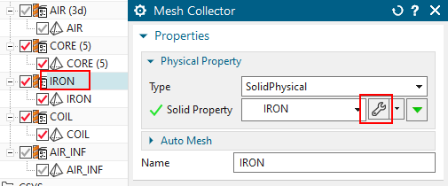
• Assign the new material to the core and also to the iron:
  

Define Stranded Coil Properties

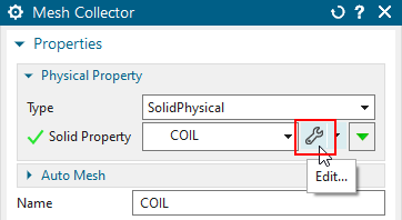
Following, we will define the properties of the coil. Even though the CAD model is a simple solid, in the simulation we want to define the electric current as flowing through individual turns.

1. Edit the Physical of the coil mesh.
   

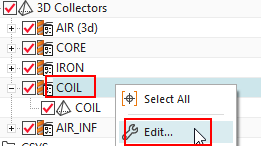
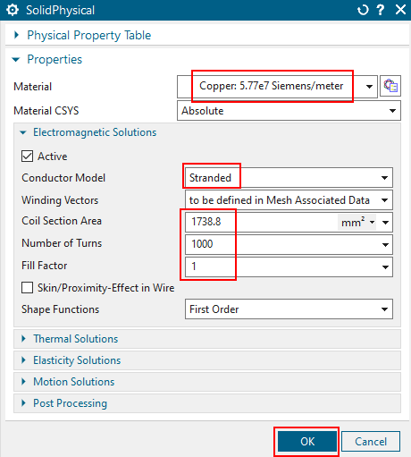
2. In the box ’Conductor Model’, set the options as follows:

3. Set ’Model’ to ’Stranded, Vectors defined in Mesh Associated Data’. This allows forcing all electric currents flowing in directions of the winding. Using this stranded method you will get a homogeneous distribution of the current over the face. In a following step we will define these directions using a spline curve.

4. At ’Material’, choose the copper from the list. (There are already some basic materials in the list because of the template that was used at creation)

5. Set ’Number of Turns’ to 1000,

6. Accept ’Fillfactor’ is 1, This setting influences the ohm resistance of the coil.

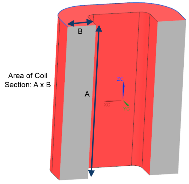
7. Set ’Coil Section Area’ to 1738.8 mm\(^{2}\). See next picture (right) for an explanation how this area is computed.
   

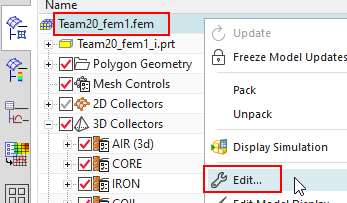
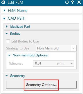
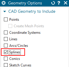
8. Define the winding directions. We first have to add the spline curve into the Fem file, which in CAD was extracted from the coil edges. To do this: edit the Fem file, click ’Geometry Options’ and activate ’Splines’ in the following window. Click OK, OK.
   

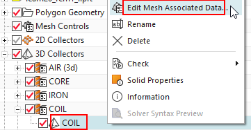
9. Now, do RMB on the mesh of the coil, Choose ’Edit Mesh Associated Data’.
   

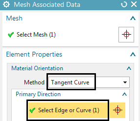
10. In the next window, set the option ’Material Orientation’ to ’Tangent Curve’ and select the spline curve for the stranded winding direction. (Blank the meshes and air volumes for easier selection)
    

11. Hint: Maybe, the spline curve is not visible. In that case, you have to fully load the CAD file of the coil. Therefore, simply make the coil the work part once.

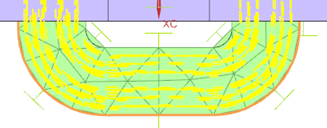
12. Hint: You can activate ’Preview’ to see the arrows pointing in positive direction. If later, current is defined on this coil, it will be forced in this direction.
    

13. Click OK, OK to finish the coil definition.

Define Infinity Properties

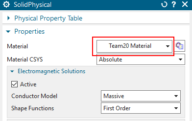
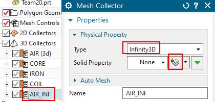
1. First, delete the existing Physical named ’AIR_INF’, because it has been automatically created with type ’SolidPhysical’, but we need one with type ’Infinity3D’: From toolbar ’Home’, ’Properties’, choose ’Physical Properties’ , select the ’AIR_INF’, which is of SolidPhysical type and click ’Delete’ and ’Close’.
   

2. Now, create a correct Physical: Edit the mesh collector ’AIR_INF’, set the ’Type’ to ’Infinity3D’, select ’Open Manager’, accept the default type ’Spherical Shell’ and key in the two values for ’Inner Radius at Shell’ and ’Shell Thickness’ as shown below. Click OK, OK.
   
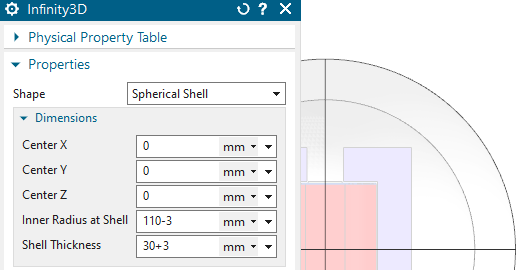
   Hint: The value ’Inner Radius at Shell’ is slightly reduced (3 mm, and the thickness value adds 3 mm to compensate) to avoid error messages like ’Bad parameters for transformation Jacobian’ that may appear from the solver. The reason for that error is that all elements of AIR_INF must be inside the two radii. But if the mesh is coarse, there may some element-edges crossing the radius value. To allow also these elements, we do that reduction.

Finish Fem File

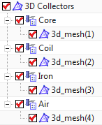
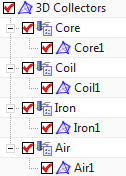
This step is not necessary if in customer defaults, the setting ’Use Polygon Body Names for Meshes and Physicals’ is activated, see chapter ’Recommended System Settings’.

• For easier post processing, click on the button ’Rename Meshes by Collectors’ from the Magnetics toolbar. That utility renames all meshes and therefore is a useful feature especially with larger models and many meshes.
  

• To finish the work in the Fem file it is a good practice to blank all meshes and unblank all polygon bodies.
  

Define Load and Constraint

1. Switch to the Sim file.
   

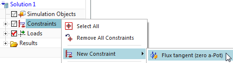
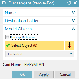
2. To keep the magnetic flux inside the air sphere, it is necessary to use a constraint ’Flux tangent’. To do so, click on ’Constraints\(\rightarrow\)’New Constraint’\(\rightarrow\)’Flux tangent (zero a-Pot)’ . Select all 8 outside faces of the air volume. Click OK.
   
   

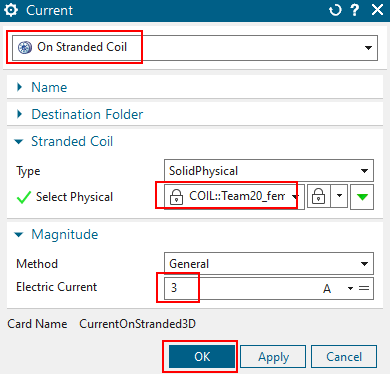
3. To create an electric current load for the coil:

   • At loads, click on ’Current’ ,

   • accept the default type ’On Stranded Coil’ and also the default Method ’General’

   • key in 3 A at ’Electric Current’.
     Hint: The positive direction of the current is defined by the spline that was selected in ’Mesh Associated Data’.

   • In the list ’Select Physical’, select the ’Coil’ and click OK to finish the creation of the coil current.
     

Solve and Post Processing

1. Solve the solution: Click on and OK. The solver will run about 20 sec.

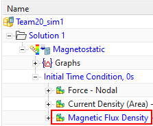
2. Post processing

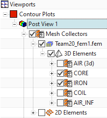
   • After the solver has finished open the results by double clicking on the ’Results’ node. Then, in the ’Post Processing Navigator’, open the node ’Solution1’ and double click on ’Magnetic Flux Density ...’.

   • Also in ’Post Processing Navigator’, hide the AIR, AIR_INF and COIL meshes by switching off their red symbols at ’Viewports’. Now the results can be seen in graphics.
     

   • The maximum Flux density in the core should be about 1.7 Tesla. The below picture shows Contour (left) and Arrows (right).
     

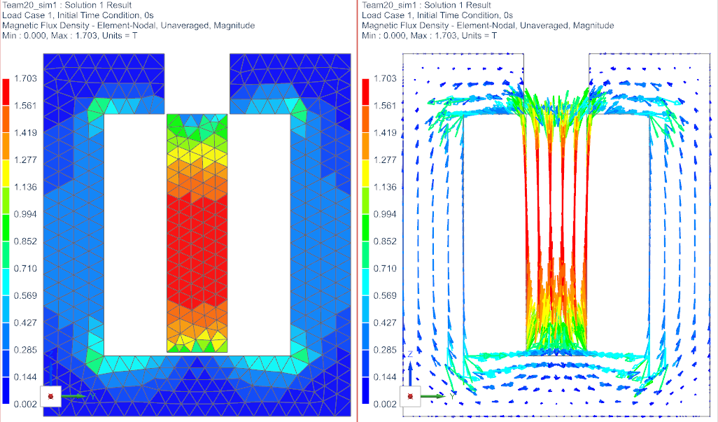
   • Tabular results, like force sum on all bodies or currents, are found at the top of the results node, as seen in the below picture. From there, the requested results can be opened and shown by ’List’ or in a graph window by ’Plot’.
     
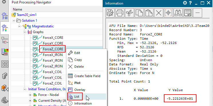
     The Z-direction force is computed to -52.2 N.
     Notice: The measured reference force is -54.4 N.

3. Variants with 3A, 4.5A and 5A
   We want to compute two other electric currents and compare them with reference measurements. Solve using the following values for the current and compare the results against measurement data (Reference data is from [TakahashiNakataMorishige]).

   • 3.0 A: Measurement: -54.4 N. Simulation: -52.2 N Deviation: 4%

   • 4.5 A: Measurement: -75.0 N. Simulation: -80.4 N Deviation: 7.2%

   • 5.0 A: Measurement: -80.1 N. Simulation: -88.5 N Deviation: 10.4%

Loss of Accuracy

Loss of accuracy normally results mainly from the mesh because of the approximation of finite elements. Thus, finer meshes or using higher order shape functions will help. On the other side, if there is an nonlinear material included, there also results some loss of accuracy from the nonlinear scheme what can be controlled by the residual tolerances. We will use both in the following.

Increasing Accuracy by Reducing Nonlinear Residuals

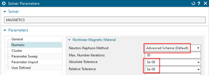
Because we us a nonlinear BH curve in one of the materials, there runs a Newton-Raphson-Iteration-loop in the solver. Tolerances control how tight our solution will be to the given BH curve. Thus, the first thing we do is reduce this tolerance by one order. Proceed as follows:

1. RMB on the solution, click ’Edit Solver Parameters’. In register ’Numeric’, box ’Nonlinear Magnetic Material’, set ’Newton-Raphson-Method’ to ’Advanced Scheme (Default)’.

2. reduce the two tolerances by one order, thus, from 5e-5 to 5e-6.
   

3. Solve again for the three currents and compare the force results. You may also notice in the logfile that the number of required iterations to converge increases.

   • 3.0 A: Measurement: -54.4 N. Simulation: -51.6 N Deviation: 5.1%

   • 4.5 A: Measurement: -75.0 N. Simulation: -75.1 N Deviation: 0.1%

   • 5.0 A: Measurement: -80.1 N. Simulation: -80.9 N Deviation: 1.0%

4. now we reduce the two tolerances again by one order to 5e-7. Solve again and find: results are the same as before. Thus, the prior tolerance 5e-6 worked already well.

5. Set the two tolerances back to 5e-6.

Increasing Accuracy by global higher Order Shape Functions

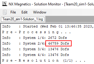
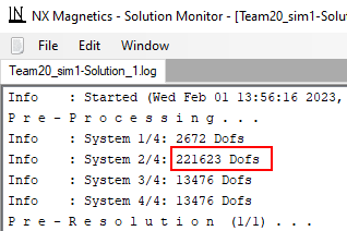
The shape functions define the approximation of the main result in the finite elements. we can increase the order without changing the mesh. We use so called hierarchical shape functions, that means, no midnode elements are necessary. Increasing the order strongly increases the number of degrees of freedom (DOFs or unknowns) in the equation system. This results in more solve time and much more necessary memory (RAM). The number of DOFs is shown in the solution monitor quite at the beginning. There are several systems shown. The relevant one is simply the largest one. The picture below shows the DOFs with the origin (first order) left and a solve with third order on the right. Notice, that the number has increased by a factor of nearly 5.

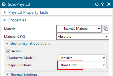
To test with third instead of first order, do this:

1. switch to the Fem file,

2. edit the physicals of Core, Iron, Air (if you want, also the coil) and for each of them

3. in box ’Electromagnetic Solutions’, set the ’Shape Functions’ to ’Third Order’.
   

4. solve again for the three currents. The solve time will increase a lot. Compare the results:

   • 3.0 A: Measurement: -54.4 N. Simulation: -54.39 N Deviation: 0.02%

   • 4.5 A: Measurement: -75.0 N. Simulation: -74.37 N Deviation: 0.84%

   • 5.0 A: Measurement: -80.1 N. Simulation: -79.64 N Deviation: 0.57%

Increasing Accuracy by local higher Order Shape Functions

Because the globally increased order of shape functions strongly increases the number of DOFs, there exists a feature for increasing that order on elements being connected to edges or faces. This is often a good compromise because the DOFs increase only slightly but the accurate shape functions are installed. For good efficiency, we should select faces or edges with sharp corners. Or simply those, where the magnetic fluxdensity changes rapidly. Proceed as follows for a test:

1. switch back to the Fem file and set all physical shape functions back to ’First Order’

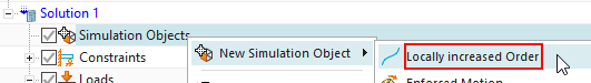
2. switch to the Sim file.

3. Create a ’Simulation Object’ of type ’Locally increased Order’
   

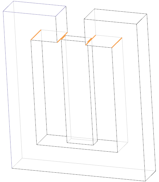
4. Accept the default type ’on Edges’ and select the 6 sharp corner edges at the upper side, where we have already seen the magnetic fluxdensity changing rapidly. These are shown in the picture.
   

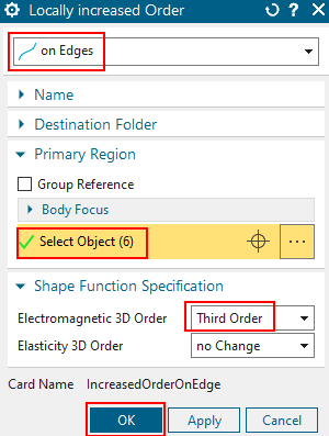
5. In ’Electromagnetic 3D Order’, set the ’Shape Function’ to ’Third Order’

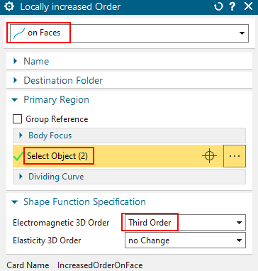
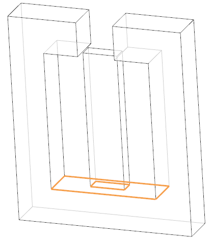
6. Create another ’Locally increased Order’, now set the type to ’on Faces’ and select the two faces at the lower side, where the flux jumps over the air-gap between the core and iron. Set the order to 3 here too.
   

7. solve again for the three currents. Notice, that we now have 53345 DOFs, only a little more than with full first order.

   • 3.0 A: Measurement: -54.4 N. Simulation: -54.96 N Deviation: 1.03%

   • 4.5 A: Measurement: -75.0 N. Simulation: -74.02 N Deviation: 1.31%

   • 5.0 A: Measurement: -80.1 N. Simulation: -78.90 N Deviation: 1.50%

Increasing Accuracy by Adaptive Meshing

To increase the result accuracy, one can also use adaptive meshing.

1. Remove the two ’Locally increased Order’ features from the model first.

2. set the core, iron and air physicals to ’Third Order’.

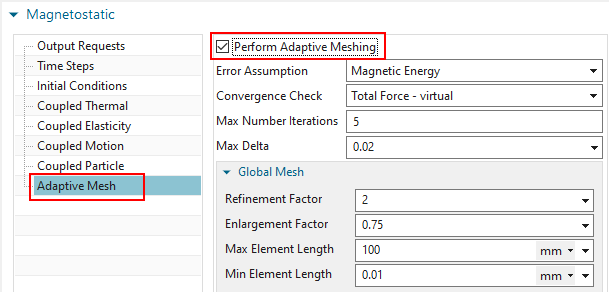
3. Activate the button ’Perform Adaptive Meshing’ in the edit solution dialogue at register ’Adaptive Mesh’ as shown in the below picture. All default settings, as seen below, can stay in many cases.
   

4. The feature adaptive meshing takes more time to solve because it reflects the results and changes the mesh to find an optimal mesh. Therefore, it should be used only with one electric current value. For the other values, it should be switched off, so the system will use the already adapted mesh. Using this, we get the final result values as shown below.

   • 3.0 A: Simulation: -55.40 N Deviation: 1.8%

   • 4.5 A: Simulation: -75.99 N Deviation: 1.3%

   • 5.0 A: Simulation: -81.32 N Deviation: 1.5%

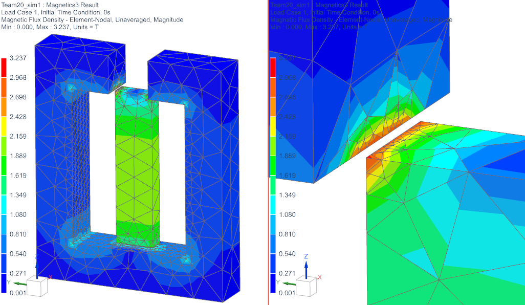
   The mesh, as it comes out of the adaptive meshing process, is demonstrated in the below picture.
   

This tutorial is complete. Save your files and close them.

Force on Magnet (TEAM 23)

In this tutorial forces between a coil and core are computed in 2D at different positions. A parameter sweep is performed to vary different CAD positions of the magnet. The model is already set up, we just have to create a second solution with a parameter sweep.

1. download the model files for this tutorial from the following link:
   https://www.magnetics.de/downloads/Tutorials/3.MagSta/3.3ForceMagnetTeam23.zip

2. unzip the archive. There will be one folder ’start’ and one ’complete’.

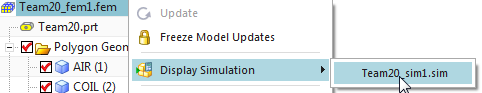
3. Start the Program Simcenter (or NX).

4. In Simcenter, click Open and navigate to folder ’complete’. Select the file ’Team23_sim1.sim’ and click OK. (Maybe you must set the file filter to ’.sim’) This file already contains the meshes, physical properties, loads and constraints.

5. Create a new Solution .

   • Key in for name ’2nd_Order_VarDis’.

   • Accept solver ’MAGNETICS’, analysis type ’2D or axisym Electromagnetics’ and solution type ’Magnetostatic’.

   • In ’Output Requests’, ’Table’, activate ’Total Force - entire (virtual)’. In ’2D’ activate ’Axisymmetric’.

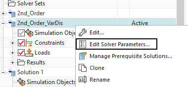
6. click RMB on the solution ’2nd_Order_VarDis’ and click ’Edit Solver Parameters’.

   • Under ’General’, switch ’Result Graphs (afu) to ’None’.

   • Under ’Parameter Sweep’, ’Perform’ assign ’One Parameter Sweep’. Continue as shown in the following window.

   

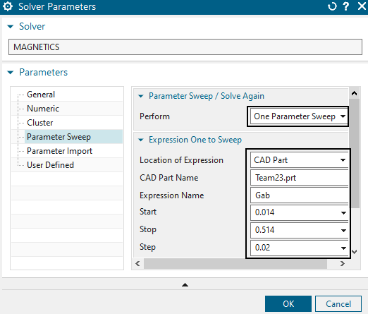
7. Explanation:

   • The ’Location of Expression’ is set to ’CAD Part’ because the location of the coil body will be variable.

   • Therefore we use ’Team23.prt’ for ’CAD Part Name’.

   • The ’Expression Name’ ist set to ’Gab’.

   • At last, the start position, the ’Step Size’ and the end position are defined.

8. Solve the ’VarDis’ solution.

9. Open the ’.VarDis.Force.txt’ file or export the table in EXEL.
   Following two plotted graphs of the forces in the Y-direction.
   
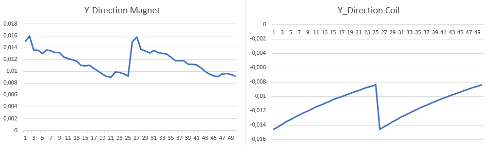
   One can see that the force becomes smaller with greater distance. This is because of the magnetic effect.