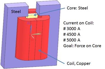
Goal of this tutorial is to learn some basics of CAD modeling in NX
or Simcenter starting from scratch. This tutorial shows very typical CAD
techniques: sketching, extruding and subtracting. If the user is
familiar with these he will be able to model much more complex geometry
in a very similar way too.
For those who directly want to see the result: The completed CAD file
for the Solenoid example can be found in this folder:
’Your
Installation’/MAGNETICS/docu/Tutorials/0.CADbasics/0.1Team20/complete If
desired, the CAD file resulting from this tutorial can be used for
starting the simulation tutorial 3D Simulation: ’Static Force on
Solenoid’
Estimated time: 45 min. Follow the steps in Simcenter:
Start the Program Simcenter ![]() (or
NX). Use Version 10 or higher.
(or
NX). Use Version 10 or higher.
In Simcenter click ’New’ ![]() ,
,
Click on register ’Model’,
in box ’Templates’ set the ’Units’ to ’Millimeters’ and select
’Model’,
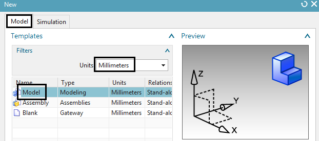
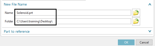
in box ’New File Name’: for ’Name’ key in ’Solenoid.prt’.
for ’Folder’ navigate to any folder you want.
Click OK. The empty part file is created and the system automatically switches into the ’Modeling’ application.
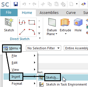
The core is a simple block positioned in the middle. We could use the ’Block’ feature for that. But we want to use a more general way: First sketching a rectangle and then extruding it to a block. Sketching means we create curves on a two dimensional plane. Following such curves are extruded or revolved and thus 3D geometry results from the sketch curves. Such features ’Sketch’ and ’Extrude’ are very comfortably and powerful. Many geometry types can be created by this way. Following we start CAD features by using the ’Menu’ command (see picture below). By doing so such features are found always at the same location. Of course most feature buttons can also be found somewhere in the toolbar where is may be faster to click. But we prefer the ’Menu’ command for this tutorial because the toolbar locations may change from user to user.
Click on ’Menu’ \(\rightarrow\)
Insert \(\rightarrow\) ’Sketch’ 
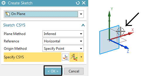
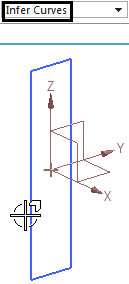
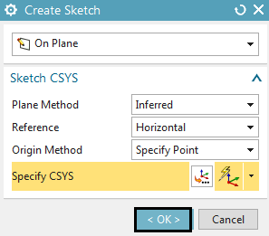
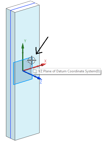
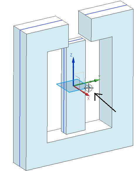
A window ’Create Sketch’ appears asking for a plane to sketch on.
Select the Y-Z (in absolute coordinates) plane as shown in the picture
below right and click OK. The sketch environment is started.
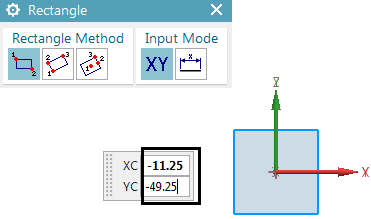
Click on ’Rectangle’  or simply key in ’r’ to use the
shortcut. A window ’Rectangle’ appears asking for the definition of the
rectangle.
or simply key in ’r’ to use the
shortcut. A window ’Rectangle’ appears asking for the definition of the
rectangle.
key in the first coordinate (-11.25 -49.25 mm) into the little entry field and press ’Return’.
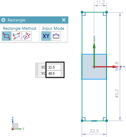
key in the second coordinate (11.25 49.25 mm) into the entry
field and press ’Return’. The rectangle is created.
Press ’Escape’ to cancel the dialog.
Click on ’Finish Sketch’  or use the shortcut ’Ctrl+Q’ to cancel
the sketch environment.
or use the shortcut ’Ctrl+Q’ to cancel
the sketch environment.
Click on ’Menu’ \(\rightarrow\)
Insert \(\rightarrow\) Design Feature
\(\rightarrow\) ’Extrude’  or simply key in ’X’ to use the
shortcut. The ’Extrude’ dialog appears.
or simply key in ’X’ to use the
shortcut. The ’Extrude’ dialog appears.
Set the selection type to ’Infer’ and select the sketch.
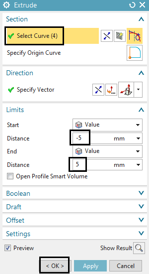
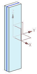
Key in the two Distance values (-5 and 5 mm) and click on OK. The block is created.
Of course it is necessary to know how to use zoom, rotate and other display options. Following is a list of useful options. Feel free testing them now:
Rotate: Click and hold the middle mouse button (MMB). Then move the mouse in the graphics area. The block will rotate.
Pan: Click and hold the middle and the right mouse button together. Again move the mouse. The block will move (pan) without rotation.
Zoom in/out: Scroll the mouse wheel to zoom in or out. Alternatively click and hold the middle and the left mouse button together.
Fit: To fit all visible geometry into the graphics area use the shortcut ’Ctrl+F’. Alternatively right click in the graphics area and from the appearing window click on ’Fit’.
Switch between shaded and wire frame display: right click in the graphics area and from the appearing window click on ’Rendering Style’. Choose from the options there: For instance ’Static Wireframe’ or ’Shaded’.
Again sketching is a convenient way for modeling the iron.
Start the sketcher by clicking on ’Menu’ \(\rightarrow\) Insert \(\rightarrow\) ’Sketch’
The window ’Create Sketch’ appears asking for the plane to sketch
on. Select the same plane as already for the core. Click OK.
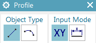
Following we are creating several line segments. Therefore the
simplest way is to use the ’Profile’ method. Click on the ’Profile’  button or simply key in ’Z’ to use the
shortcut. A window asking for coordinates appears.
button or simply key in ’Z’ to use the
shortcut. A window asking for coordinates appears.
 .
.
Key in the following x,y coordinates into the little entry field.
To begin a new x,y entry click  . Press ’Tab’ to switch between x and y
and press ’Return’ after each coordinate pair. Use these x,y value
pairs:
. Press ’Tab’ to switch between x and y
and press ’Return’ after each coordinate pair. Use these x,y value
pairs:
-13.5 75 , -63.5 75 , -63.5 -75 , 63.5 -75 , 63.5 75 , 13.5 75
There appears a profile as shown below.
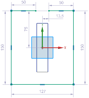
Press ’Escape’ to cancel the dialog.
Finish the sketch
The following extrude feature is a little special because we use it with an ’Offset’ option. This option allows creating a solid body from a (non closed) profile. In many cases this is a convenient way to create geometry.
Click on ’Menu’ \(\rightarrow\)
Insert \(\rightarrow\) Design Feature
\(\rightarrow\) ’Extrude’ . The ’Extrude’ dialog
appears.
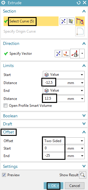
Set the selection type to ’Infer’ and select the new sketch.
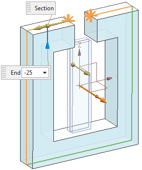
Key in the two Distance values (-12.5 and 12.5 mm) and check the direction of the specified blue vector (your iron geometry should look like the one in the picture below).
Click on the box ’Offset’ to make such options visible.
Set the ’Offset’ to ’Two Sided’ and key in 0 and -25 mm in the field. (Attention: Sometimes you may need the opposite: 25 instead of -25. Please check your iron geometry against the one in the below picture)
Click on OK. The iron geometry is created.
For the coil we also use the sketch/extrude method and we also exploit the ’Offset’ option. It can be seen that these features are really useful for many types of geometry.
Start the sketcher by clicking on ’Menu’ \(\rightarrow\) Insert \(\rightarrow\) ’Sketch’
The window ’Create Sketch’ appears. Now for the coil, select the
plane (X-Y) that is perpendicular to the core and iron plane.
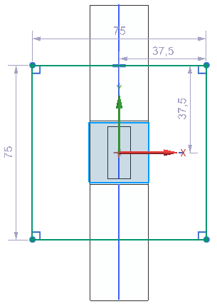
Following we are sketching a rectangle first and then use the fillet function to create circles at the four corners.
Click on ’Rectangle’ or simply key in ’R’ to use the
shortcut. The window ’Rectangle’ appears asking for the definition of
the rectangle.
Key in the first coordinate (37.5 37.5 mm) into the little entry field and press ’Return’.
Key in the second coordinate (-37.5 -37.5 mm) into the entry field and press ’Return’. The rectangle is created. See picture below left. Press ’Escape’ to cancel the dialog.
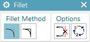
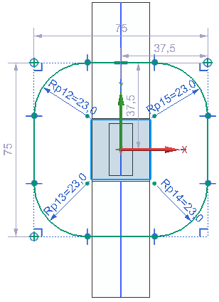
Click on ’Fillet’  or simply key in ’F’ to use the
shortcut. A window ’Fillet’ appears asking for line pairs.
or simply key in ’F’ to use the
shortcut. A window ’Fillet’ appears asking for line pairs.
Select the two lines of a corner and key in the radius 23 mm.
Press ’Enter’ and the fillet is created.
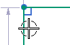
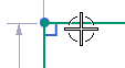
Repeat the fillet creation for all four corners of the rectangle.
The result is shown in the below picture right.
Finish the sketch
For extruding the coil we again use the ’Offset’ option.
Click on ’Menu’\(\rightarrow\)Insert\(\rightarrow\)Design Feature\(\rightarrow\)’Extrude’ . The ’Extrude’ dialog appears.
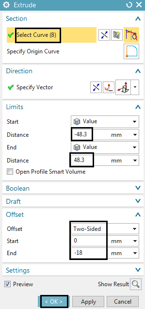
Set the selection type to ’Infer’ and select the coil sketch.
Key in the two Distance values (-48.3 and 48.3 mm).
Click on the box ’Offset’ to make such options visible.
Set the ’Offset’ to ’Two Sided’ and key in 0 and -18 mm in the field. (Hint: In some cases you will need 18 instead of -18.)
Click on OK. The coil geometry is created.
Later in the simulation we will define winding directions for this coil. There it is necessary having one joined curve instead of several pieces. Therefore proceed as follows: Click on Menu\(\rightarrow\)Insert\(\rightarrow\)Associative Copy\(\rightarrow\)’Extract Geometry’. The ’Extract Geometry’ dialog appears. Check the type is set to ’Composite Curve’. Select the 8 sketch curves and click OK. The new curve is created.
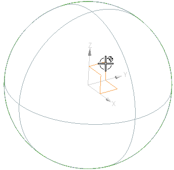
In Electromagnetics and also in Flow simulations it is necessary to model the air or fluid volume. In many cases this can be a simple sphere or a box. The detailed air volume for later meshing results from a subtraction of all solenoid volumes from that air volume. For easier meshing we will finally subdivide the face of the sphere. We model such a sphere in the following.
Click on ’Menu’ \(\rightarrow\)
Insert \(\rightarrow\) Design Feature
\(\rightarrow\) ’Sphere’  . The ’Sphere’ dialog appears.
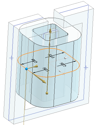
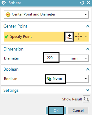
Click on the ’Point Dialog’ and key in the center point coordinate (0 0 0).
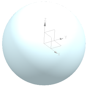
Key in 220 mm at ’Diameter’ and click OK. The sphere is
created.
Click on ’Menu’ \(\rightarrow\)
Insert \(\rightarrow\) Combine \(\rightarrow\) ’Subtract’  . The ’Subtract’ dialog
appears.
. The ’Subtract’ dialog
appears.
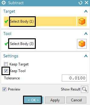
Click on ’Target - Select Body’ and select the sphere volume.
Click on ’Tool - Select Body’ and drag a window over everything. The three solenoid bodies are selected.
Activate the button ’Keep Tool’ and click OK. The operation is
performed.
Click on ’Menu’ \(\rightarrow\)
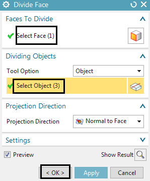
Insert \(\rightarrow\) Trim \(\rightarrow\) ’Divide Face’ ![]() . The ’Divide Face’ dialog appears.
. The ’Divide Face’ dialog appears.
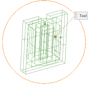
Click on ’Faces to Divide - Select Face’, set the selection filter to ’Single Face’ and select the spherical face.
Click on ’Dividing Objects - Select Object’ and select the three planes of the datum coordinate system.
Click OK and the face subdivisions are performed.
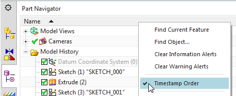
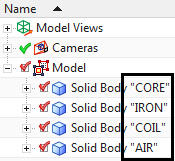
Later in the simulation working with speaking names is quite helpful. Therefore we want to assign names to the bodies. Such bodies will result in so called ’Polygon Bodies’ later and these will be used for creating finite element meshes.
In the ’Part Navigator’ right click on the grey border (see picture below) and deactivate ’Time Stamp Order’. Now bodies are shown in the navigator instead of the creation order of CAD features.
Use RMB on each of them, chose ’Rename’ and assign speaking
names.
The tutorial is complete. Save your parts and close them.