In this tutorial we analyze a permanent magnet electric motor in 3D. For motion we use the Sliding Motion technique. A Fem and Sim file are already created and in this exercise we walk through the existing model to check and explain the used features.
In this tutorial the motor is set up in 3D but also in 2D. Both
models base on a 2D skeleton geometry. The skeleton contains only basic
dimensions and allows geometry updates into both simulation models. For
working on such motors in practice we recommend the process shown here:
Having both 2D and 3D simulation models in parallel. Because in 2D
solving runs much faster, it is a good idea to first test many things
using the 2D model and when this runs fine, set up the 3D model in the
same way and investigate the 3D behaviour.
Previous tutorials already have shown features for 2D models, so we now
will concentrate on the 3D model. The following files contain all
features for the set up of the model. There is also a youtube video (click
Link) available for this example.
Download the model files for this tutorial from the following
link:
https://www.magnetics.de/downloads/Tutorials/6.CouplMotion/6.7Motor3D.zip
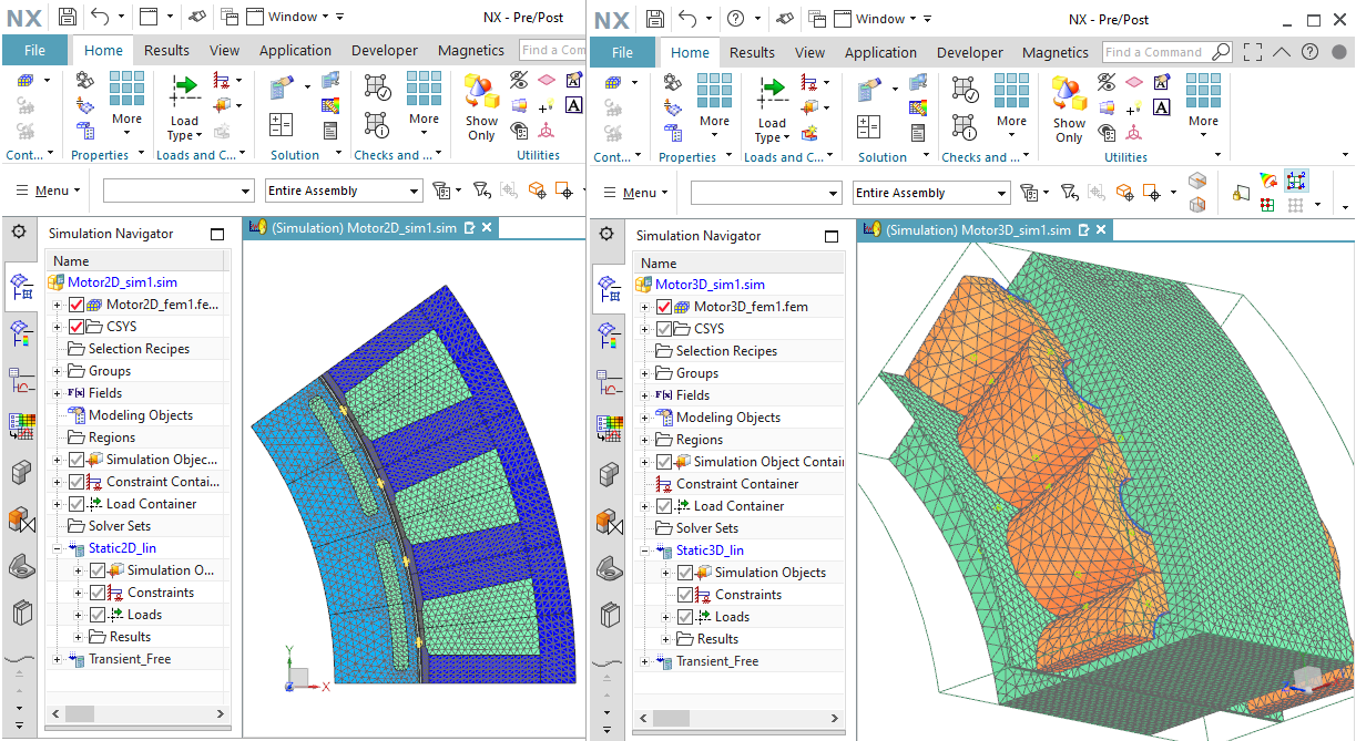
Open the file ’Motor3D_sim1.sim’.
Change the displayed part to the Fem file to check the following steps.
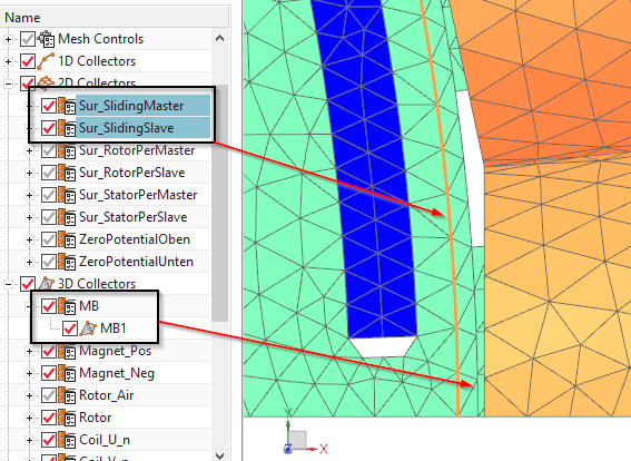
In models that use the Sliding Surface technique, there must be such two contacting surfaces that later will slide. Normally this sliding is designed into the air gap of the motor. If a motor has two such air gaps it is also possible to define two such sliding surface pairs. It is important that the sliding surfaces have the following properties:
One surface must be connected to the rotor and the other surface must be connected to the stator. At the contact, the two surfaces do NOT share the same nodes. Mesh Mating Conditions using the option ’Free Coincident’ allow for such a condition. Following we call such two surfaces ’Sur_SlidingMaster’ (the one at the stator) and ’Sur_SlidingSlave’ (the one at the rotor). The software will create link constraints between the edges of these two.
The surface must be meshed in structured way. So, when rotation appears, the link condition can snap from one element edge to the following. The optimal step size is exactly the element size, but rotor positions in between such snap points are also possible, because the neighbouring 3D elements are allowed to be slightly deformed to meet such positions.
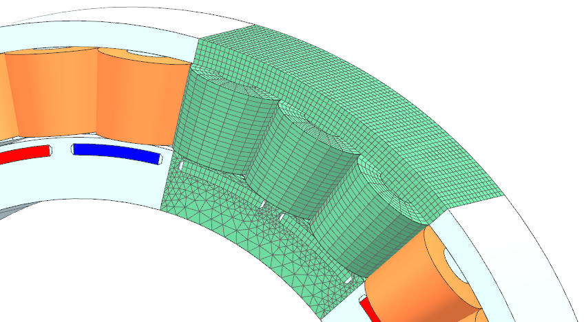
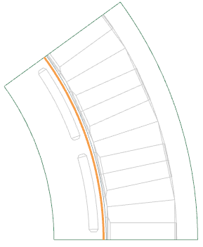
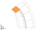
The following picture shows the position of the sliding surfaces in
the tutorial motor. Also there is shown the neighbouring 3D element
layer, called ’MB’. In this layer we allow the deformation of elements.
Also this layer is used to compute the torque results using the maxwell
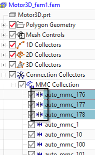
stress tensor technique. The right picture below shows the special Mesh
Mating Conditions on those faces that belong to the sliding surface. The
symbols show their type ’Free Coincident’.
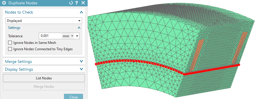
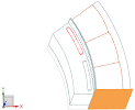
Also, for checking the sliding surface conditions for correctness, it is
a good idea to ask the model for duplicate nodes. This check must show
all nodes at the sliding surfaces highlighting. See picture below.
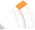
Of course, to keep simulation time as short as possible, one should exploit the periodicity that most motors have. Therefore, we will model a link constraint between the right and left section faces of the motor segment. The following recommendations are given:
These section faces are meshed at the very beginning of the meshing process using the ’2D Dependent’ meshing feature.
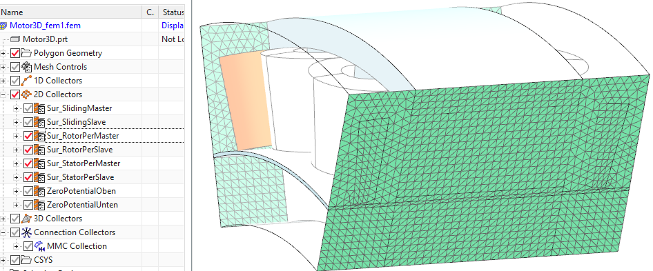
The resulting 2D meshes at these periodicity faces will later be referenced in a link condition. Therefore we will call such 2D meshes as follows:
’Sur_RotorPerMaster’: The faces on the right (master) side,
belonging to the rotor.
’Sur_RotorPerSlave’: The faces on the left (slave) side,
belonging to the rotor.
’Sur_StatorPerMaster’: The faces on the right side, belonging to
the stator.
’Sur_StatorPerSlave’: The faces on the left side, belonging to
the stator.
Most specific definitions for the sliding surface technique are in a simulation object. So we take a closer look on that side.
Change the displayed part to the Sim file for the following steps.
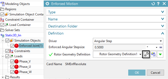
Edit and check the simulation object ’Enforced Joint(1)’. Notice its Card Name, it is a ’SMEnfRevolute’, meaning an ’Enforced Revolute by Sliding Motion’.
Only the ’Driver’ and the step size (of Velocity) are defined in this dialogue. All remaining definitions correspond to the geometrical description of the rotor and are stored in a modeling object ’Rotor Geometry Definition1’.
Edit that modeling object to see its properties. There are
several boxes to define the geometry. We walk through them
following.
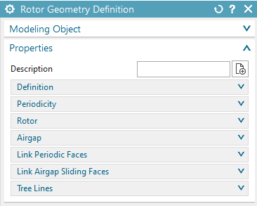
The ’Definition’ box gives some information about the orientation
of the model. A button ’Show Orientation Image’ can be set. The model
must be oriented in this way: Rotation is about global X and the start
position must be aligned with X.

The ’Tolerance Factor for Links’ must sometimes be modified.
It must be increased (use factor 10) if a message like the
following appears in the solution monitor:
Warning : Could not find edge corresponding to reference edge ...
Error : Constraint Link: bad correspondance of number of edges
...
It should be decreased, if this message appears:
Warning : Edge ... (...) already exists with tolerance ...
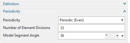
In box ’Periodicity’ there must be chosen between periodic (even) and anti periodic (odd) conditions. The ’Number of Element Divisions’ on the sliding surface as well as the ’Model Segment Angle’ are defined here.
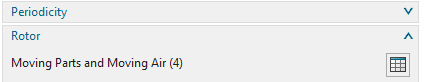
box ’Rotor’ must be used to define the ’Moving Parts and Moving
Air’.
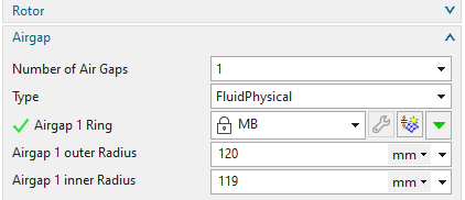
In box ’Airgap’ the ’Number of Air Gaps’ is defined as well as the Physicals of the ’Airgap 1 Ring’. Also the two radii are there defined.
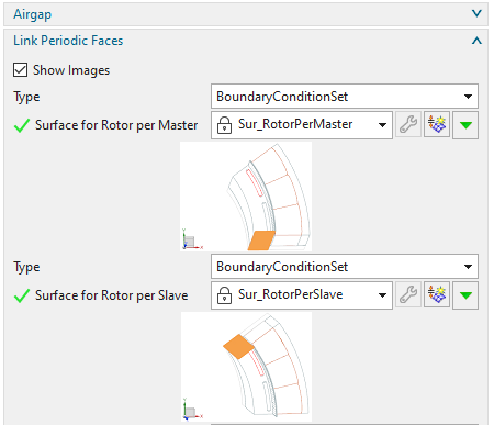
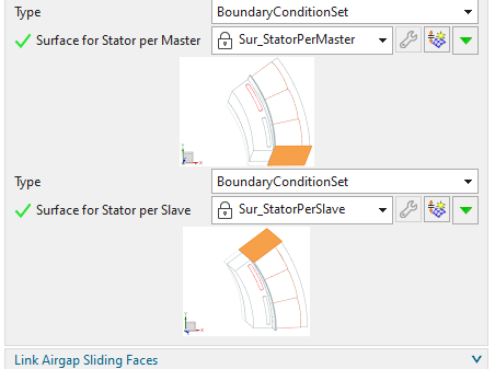
Box ’Link Periodic Faces’ must be used to define the four
previously already meshed 2D dependent meshes on the rotor and the
stator, master and slave sides. The naming here corresponds to the names
we used in the previous text. Such 2D meshes must be assigned a physical
of type ’BoundaryConditionSet’.
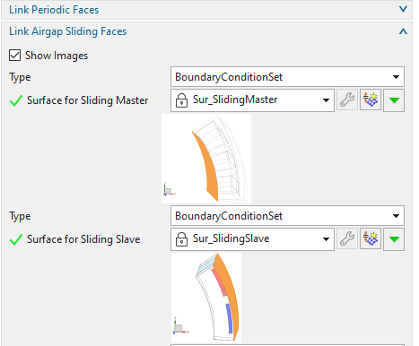
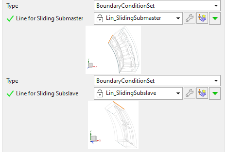
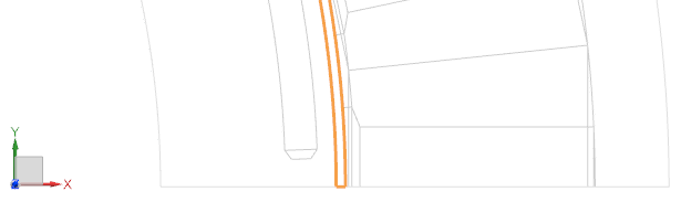
Box ’Link Airgap Sliding Faces’ defines the two previously meshed
sliding surfaces on the rotor and the stator. Also, the two lines
’Lin_SlidingSubmaster’ and ’Lin_SlidingSubslave’ are defined here.
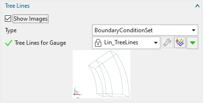
Finally, the box ’Tree Lines’ can be used to define the
previously meshed main edges of the rotor and the stator. This selection
is only necessary if the gauge type ’Tree, Cotree’ is used (in case of
sliding surface motion and linear material properties).
We recommend the following process for the meshing of 3D motors with the sliding surface technique.
Create the CAD model in the correct orientation.
Include the air gap in the CAD model. For better accuracy of
torque results, the air gap should be divided into three layers.
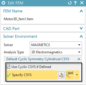
In ’Edit FEM’, set the ’Default Cyclic Symmetry Cylindrical CSYS’ to absolute (see picture above, right). This allows the 2D dependent meshes to become more robust.
Start with the automatic creation of the Mesh Mating Conditions. First create all with option ’Glue Coincident’. Then locate those conditions at the sliding surface and set these to option ’Free Coincident’.
Then create the 2D dependent meshes at the two segment sections. Try as much as possible using the structured mesh option there. This is a bit sensitive, because the link constraints will not work, if these 2D dependent meshes are not accurately positioned. Put the meshes into mesh collectors. Assign names, as they are later referenced (Sur_RotorPerMaster, ...).
Then create the sliding surface mesh at the stator side (Sur_SlidingMaster). Use the ’2D Mapped’ mesh command for that. When defining the number of elements along the circular edge, keep this number for later use in the modeling object for the rotor definition.
Now create the 3D meshes at the air gap.
Next create all other 3D meshes. Easiest way is to use only
tetrahedral elements, but also hex and pyramid transitions can be
used.
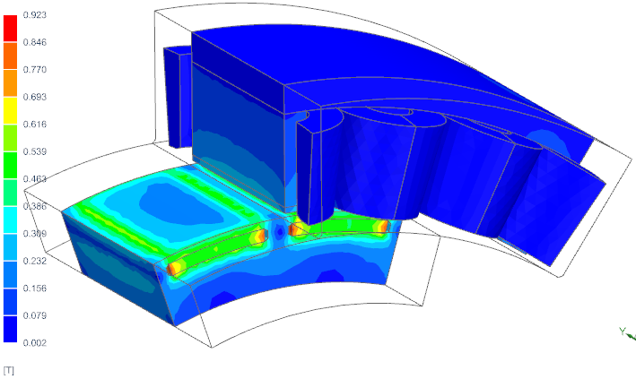
The remaining features in this model are not very special: Meshes,
mesh mating conditions, materials, electric current loads, solution
properties. Of course, the solve time for this 3D model is much higher
than for the 2D case. Particular if there is nonlinear material included
this is the case. We want to mention that also dynamic solutions are
possible with this Sliding Motion feature. Results show either tabular
graphs with torque, losses and others or plot results showing field
results with time steps and motion. Following we present some result
illustrations.