In this tutorial we analyse a permanent magnet electric motor in 3D. For motion we use the General Motion technique. A Fem and Sim file are already created and in this exercise we walk through the existing model to check and explain the used features.
Download the model files for this tutorial from the following
link:
https://www.magnetics.de/downloads/Tutorials/6.CouplMotion/6.9Motor3DGenMot.zip
Open in Simcenter the file ’Motor.prt’.
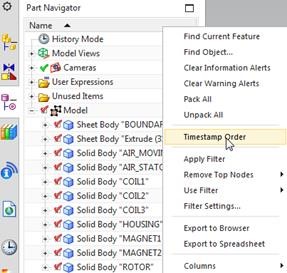
For checking this CAD file, use the modeling application. In the
Part-Navigator deactivate the ’Time Stamp’. This setting allows to see
the volumes and sheet bodies regardless of their creation history.
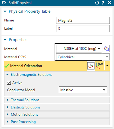
For the General Motion feature there must be a separation between
moving and stationary parts. All nodes that belong to the moving parts
will be rotated during the analysis process. The area between moving and
stationary parts will be meshed newly at every time step. To keep this
process efficient one should try to only have a small area for that mesh
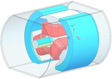
update. In many cases – and also in this example – a small air gap
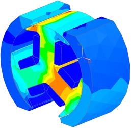
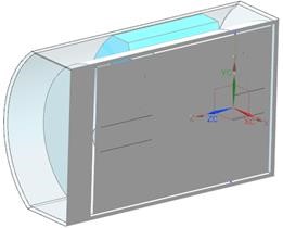
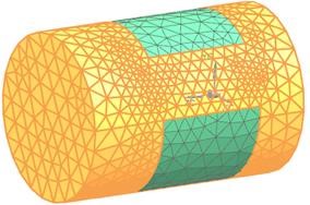
around the moving parts can be used for the mesh update. When sectioning
the view the air gap that surrounds the rotor can be seen.
Open the Fem file Motor_fem1.fem. All meshes are very coarse. Let’s check the meshes that reside in the file.
First check the Rotor mesh and the three coil meshes. There is
nothing very special here.
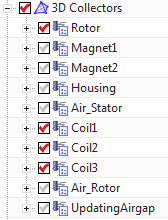
Next check the ’Air_Rotor’ mesh. This mesh represents the
rotating part of air. All rotating meshes are referenced in the Sim file
by the Simulation Object ’Enforced Revolute by General Motion’.
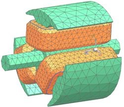
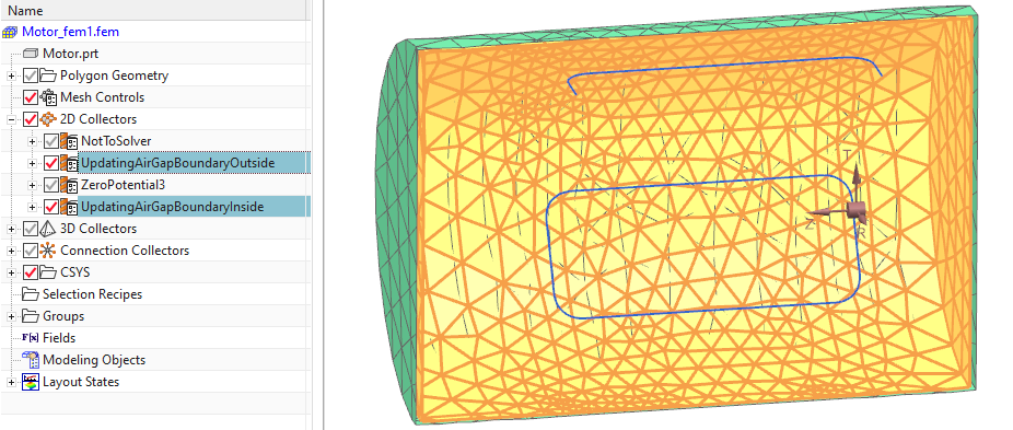
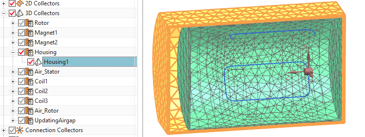
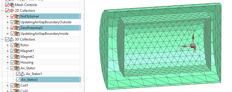
Around these rotating parts there is the updating gap (picture
below). That gap is bounded by 2D meshes. When solving, the system will
automatically create and update that gap mesh using a ’Solid from Shell
Mesh’ type mesh. This mesh will update with each time step. The boundary
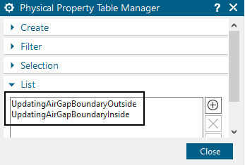
meshes reside in two mesh collectors: ’UpdatingAirGapBoundaryOutside’
and ’UpdatingAirGapBoundaryInside’. The number and names of these
boundary meshes can vary as needed.
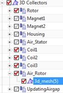
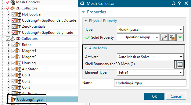
Notice the 3D mesh collector ’UpdatingAirgap’. Edit and open the
box ’Auto Mesh’ and see that this collector has activated ’Auto Mesh at
Solve’. In ’Shell Boundary for 3D Mesh’ there are the two Physicals of
the boundary meshes selected. That way, the air gap mesh will be
recreated at each solve step.
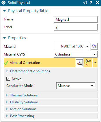
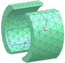
Next look at the magnets. They use cylindrical coordinate systems
and point in opposing directions.
And check the housing, a thin walled metal geometry.
The Air_Stator mesh collector represents those air parts that do
not move. This is made by two 3D-meshes.
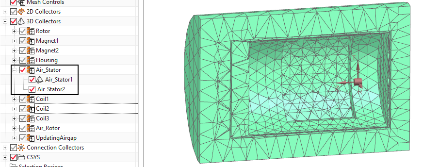
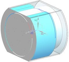
One of the above two Air_Stator meshes is created by the function
’3D Mesh from Shells’ and the used shells are shown here: One shell mesh
uses a simple ’Not to Solver’ Physical and the other a ’Zero
Potential’.
Change to the Sim file now.
We use a Magnetostatic solution type. Magnetodynamic transient is possible also.
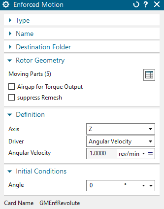
See the Enforced Revolute joint feature: We rotate about Z and
Angular Velocity set to 1 rev per min.
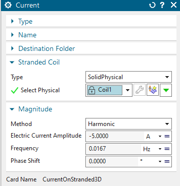
All currents are set to harmonic as shown above for coil 1. You can change these conditions to your needs.
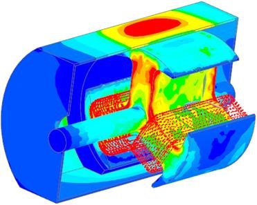
Solve the solution for as many steps as you desire.
Postprocess your results.