 The following tutorial shows such an
application. Example is the induction motor ’TEAM30’ that is one of the
Compumag reference models.
The following tutorial shows such an
application. Example is the induction motor ’TEAM30’ that is one of the
Compumag reference models.In some cases there is motion, but the geometry remains constant.
This is the case for instance if the rotor is a simple tube as in the
following example. In such situations the simulation is much simpler,
because all movements can be handled solver internally, thus we can use
the feature ’Conductor Motion const Shape’. For comparison we first
solve this model with a moving band and then again with conductor
motion.
The following tutorial shows such an
application. Example is the induction motor ’TEAM30’ that is one of the
Compumag reference models.
Download the model files for this tutorial from the following
link:
https://www.magnetics.de/downloads/Tutorials/6.CouplMotion/6.1InductionMotorTeam30.zip
Open the file Team30.prt.
Create a new Sim and Fem file(Non-Manifold) from ’Magnetics’ Toolbar.
Use solver MAGNETICS, Analysis type ’2D or axisym Electromagnetics’ and Solution Type ’Magnetodynamic Transient‘.
Name the solution ’Hochlauf’ (e.g. start-up).
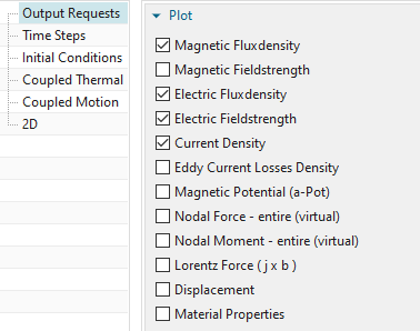
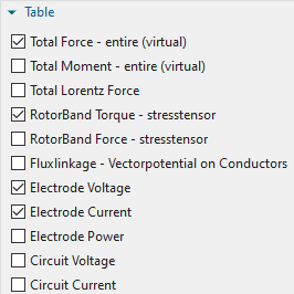
Activate the desired data in Output Requests (here we activate
’Rotorband Torque’)
In time steps, set the ’Time Increment’ to 1/2160 and the ’Number of Time Steps’ to 10.
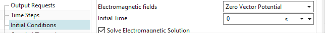
Set the Electromagnetic fields as shown in the ’Initial
Conditions’ options.
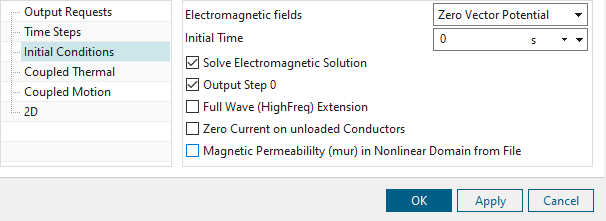
Click OK.
Switch to the FEM file.
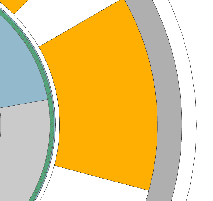
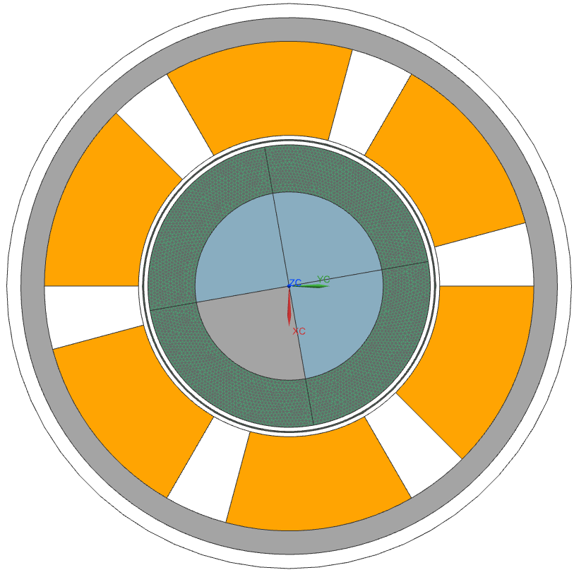
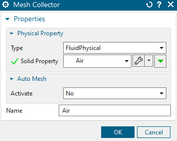
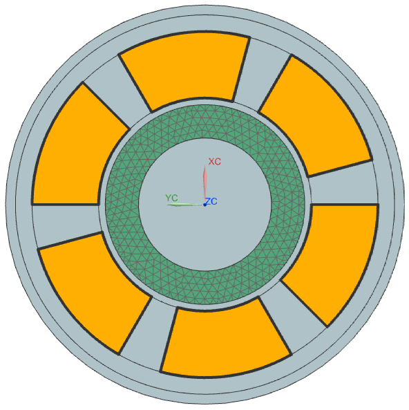
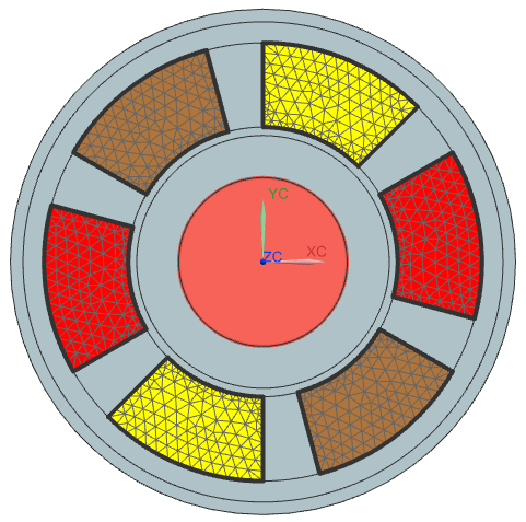
Mesh the inner part of the air gap (quads, 0.75mm) and use
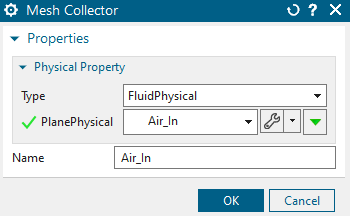
FluidPhysical and ’Air’.
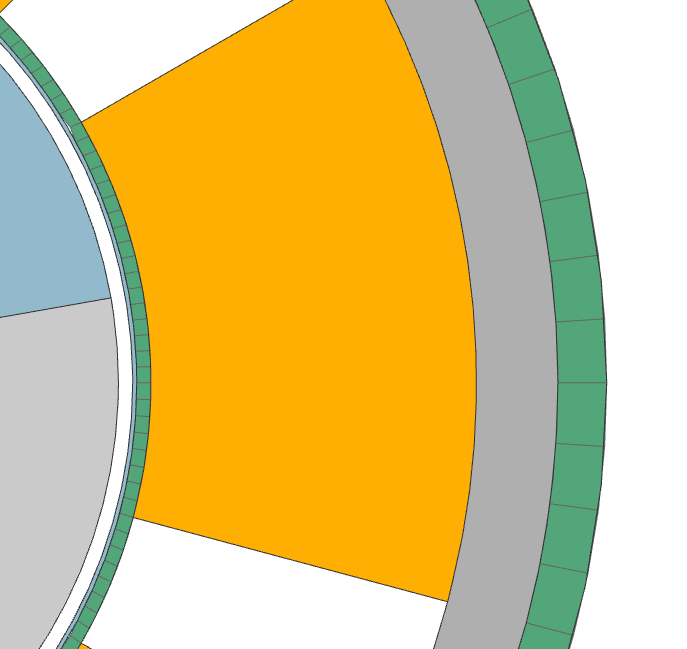
The outer air consists of 3 different quad meshes. Mesh the inner
circle with 1mm and the outer circle with 4mm. Mesh the gaps between the
coils with a 2D Mapped Mesh and the Element Size of 2mm. Assign the
fluid Physical and select the material ’Air’.
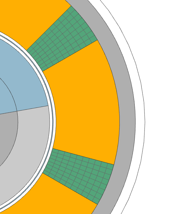
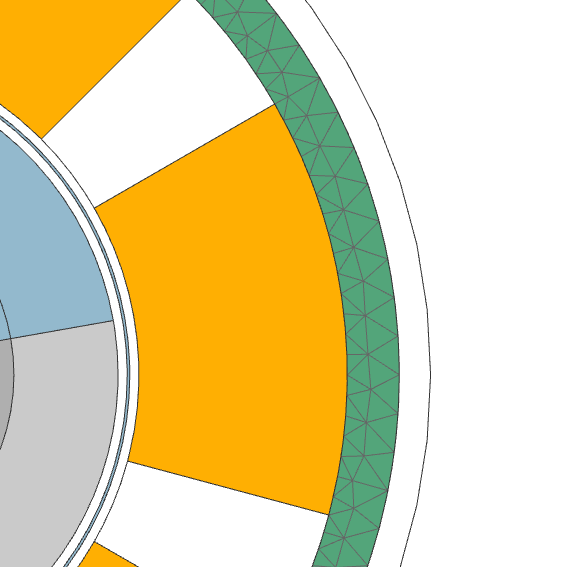
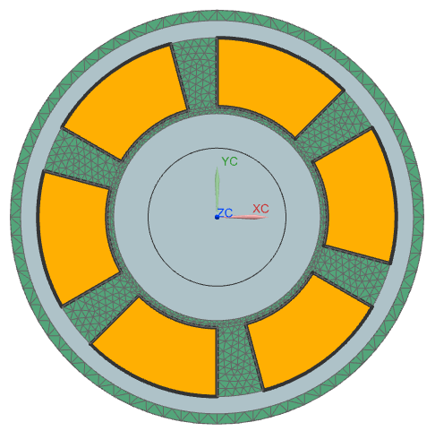
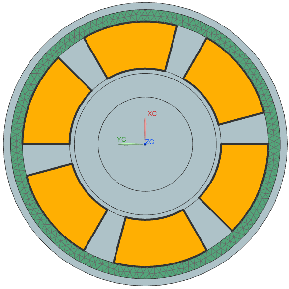
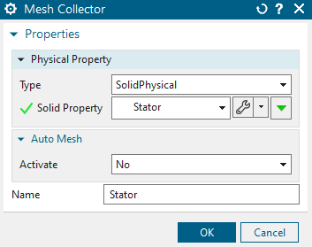
Mesh the Stator with tri meshes and an element size of 2mm.
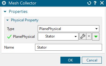
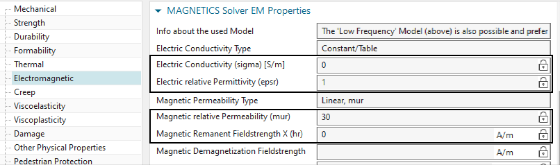
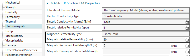
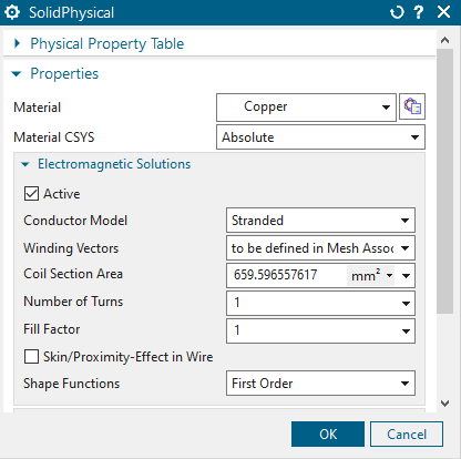
Edit the physicals and create a new Material with the name
’Team_30_Steel_Non_Con’. In ’View’ select All Properties and add the
electromagnetic properties as seen in the picture below.
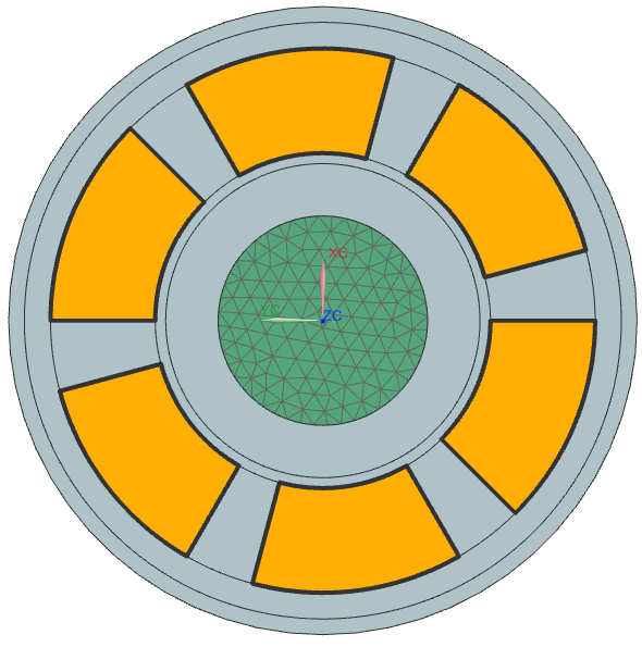
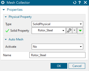
Mesh the Rotor_Steel with tri meshes and an element size of
0.75mm.
Edit the physicals and create a new Material with the name ’Team_30_RotorSteel’
In ’View’ select ’All Properties’ and add the electromagnetic
properties as seen in the picture below.
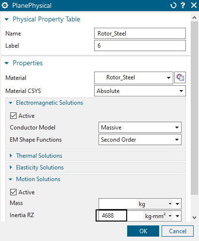
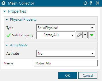
Mesh the Rotor_Alu (tri, 0.75mm) and choose material Aluminum:
3.8e7 Siemens/meter. Set the Inertia RZ to 4688\(kgmm^{2}\)
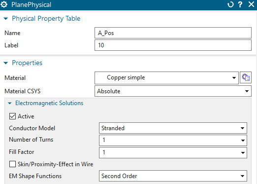
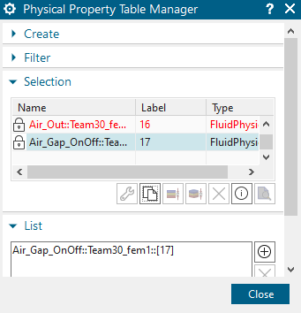
Mesh all the coils (tri, 0.75mm) and for each coil set the
physical as shown in the picture below.
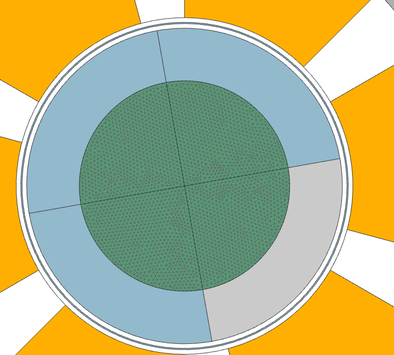
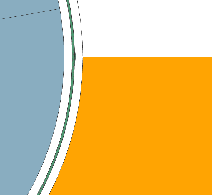
Mesh the Airgap (tri, 1.69mm) and choose fluid and Air.
We are done with the FEM file.
Change the window to the Sim file.
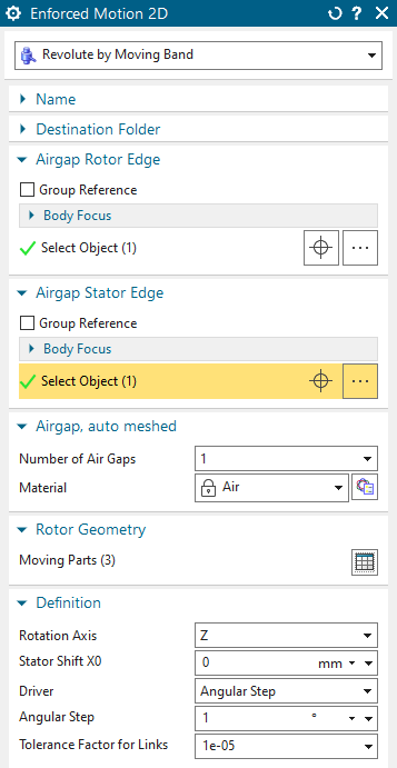
In this section we will use a Moving band to allow the rotor to move.
Create a simulation object ’Enforced Motion 2D’ and select type
’Revolute by Moving Band’. Select the ’Airgap Rotor Edge’ and the
’Airgap Stator Edge’. Use the same setting as seen in the picture
below.
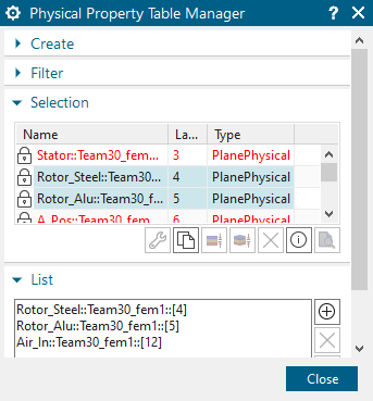
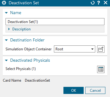
Create another Simulation object, ’Deactivation Set’ and select
the airgap in ’Deactivated Physicals’:
Create a Constraint of type ’Flux Tanget’ and select the outside edge of ’Air_Out’.
Lastly we create the Loads.
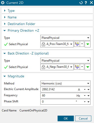
Create a Current and select the settings as below.
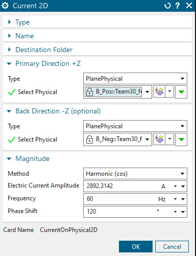
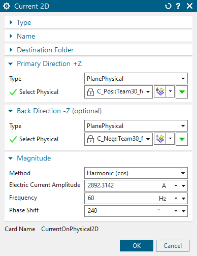
Create two more currents ’B’ and ’C’. Select the same settings
and add a phase shift of \(120^\circ\)
for ’B’ and \(240^\circ\) for
’C’.
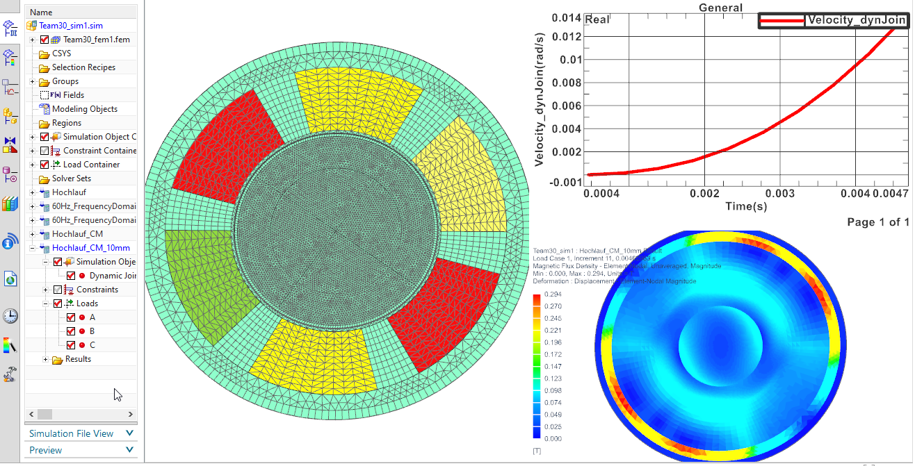
Solve the solution.
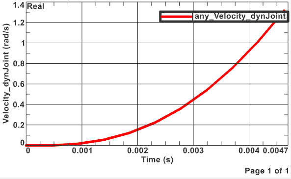
Display the graph results for the velocity. This should look like
in the folowing picture:
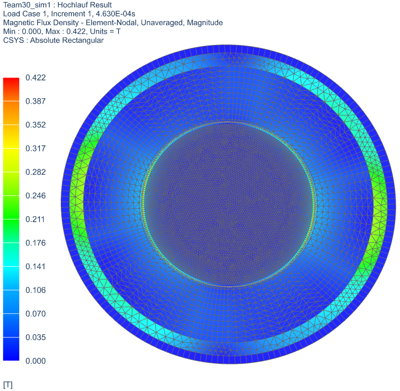
This picture shows the ’Magnetic Flux Density’ of the
motor:
Clone the solution
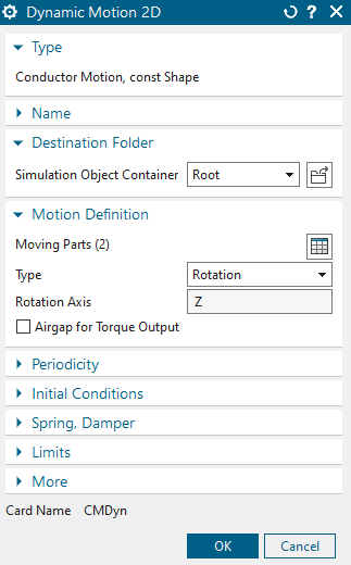
Instead of using the Moving band, we are now going to use the type ’Conductor Motion’.
Delete the two existing simulation objects. Create then a new one
of type ’Dynamic Motion 2D’ with the following settings:
Solve the solution.
The result graphs should match with the graphs of the ’Hochlauf’ solution. The tutorial is completed.
In this simulation, we are going to look at the same motor but in a 3 dimensional space.
Open the file Team30_3D.prt.
Create a new Sim and Fem file(Non-Manifold) from ’Magnetics’ Toolbar.
Use solver MAGNETICS, Analysis type ’3D Electromagnetics’ and Solution Type ’Magnetodynamic Transient‘.
Name the solution ’Hochlauf’ (e.g. start-up).
Activate the desired data in Output Requests (here we activate ’Rotorband Torque’)
In time steps, set the ’Time Increment’ to 1/2160 and the ’Number of Time Steps’ to 10.
Set the ’Electromagnetic fields’ as shown in the ’Initial
Conditions’ options.
Click OK.
Switch to the FEM file.
Mesh the ’Air’ using tets (3.2/2 mm)
Mesh the ’Stator’ with tets and an element size of 5.25/2 mm.
Add the same material to the ’Stator’, which was used in the 2D
simulation.
Mesh the ’Rotor_Alu’ with tets and use the element size of 5.1/2mm.
Add the same material to the ’Rotor_Alu’, which was used in the
2D simulation.
Mesh the ’Rotor_Steel’ with tets and use the element size of
7.67/2 mm and use the same material, which was used in the 2D
simulation.
Mesh every coil using tets and an element size of 6.04/2 mm. Set
the physicals for each coil as shown in the picture below.
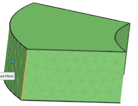
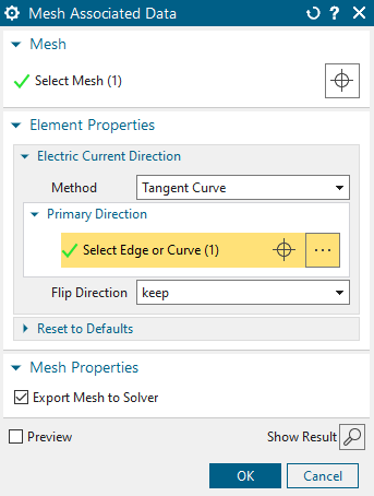
Edit the ’Mesh associated data’ and select one of the vertical,
outer lines (highlighted edge in the picture below).
We are done with the FEM file.
Change the window to the Sim file.
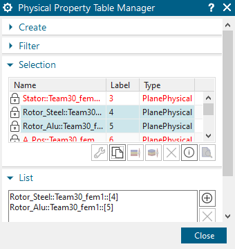
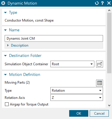
Create a simulation object ’Dynamic Motion’ of type ’Conductor
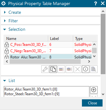
Motion’.Select the moving parts as seen in the picture below.
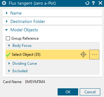
The only constraint we use here is a ’Flux Tangent’. Select all
outside faces (35 in total).
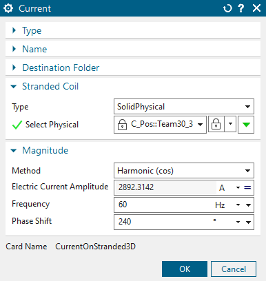
Lastly, we create the loads. Every pole has a positive and a negative current, so we have to add a load of 2892.3142 amps to the positive and a load of - 2892.3142 amps to the negative coil.
A: Phase shift of \(0^\circ\)


B: phase shift of \(120^\circ\)

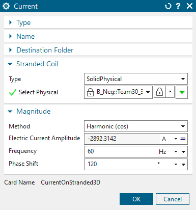
C: phase shift of \(240^\circ\)

Solve the solution. The results should be similar to the ones from the 2D simulation.