In this tutorial an induction or asynchronous motor is analysed. In part one we use a frequency domain analysis in order to provide quick results. Such frequency domain analysis provides settled situations of dynamic problems with harmonic behaviour. However, the frequency domain analysis also has some disadvantages, such as: nonlinear material properties can be simulated only with reduced accuracy; and same-wise also no permanent magnets are possible to be simulated.
In a second part we will analyse the temperatures in the motor.
Herein, we will perform a sweep over the full operating range.
In a third part we will use a time domain analysis to solve this problem
at one operating point. We will see that the resulting torque agrees
nicely to the prior frequency analysis. In time domain we can include
accurate nonlinear material effects; also the inclusion of permanent
magnets would be possible, but is not needed here. The time domain
analysis works quite similar as the prior examples of this
document.
After that we want to use time domain analysis to investigate the
starting behaviour of the motor. We find that the resulting velocity
after some time agrees to the synchronous velocity.
Finally we show a 3D model of the induction motor with simulation in
frequency domain. This simulation shows very similar results as the 2D
simulation of part one but it would additionally allow to study end
effects and other 3D specific effects.
In the frequency domain solutions results come out without rotor motion.
Therefore they depend also on the relative position of rotor to stator
bars. To check for this influence one could simulate at different rotor
angle positions. The 2D CAD model has an expression to control that.
For the basic setup follow these steps:
Download the model files for this tutorial from the following
link:
https://www.magnetics.de/downloads/Tutorials/6.CouplMotion/6.6InductionMotor3kW.zip
Open the file InductionMotor_3kW.prt.
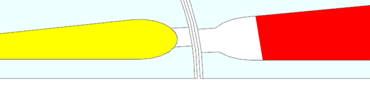
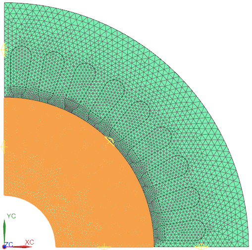
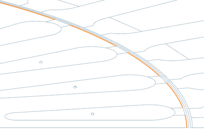
Notice the air gap in the next picture: There is one layer for
the inner mesh, one for the outer mesh and the middle layer is without
geometry. Here the solver will create a Moving Band mesh by
himself.
Create a new Sim and Fem file.
Use solver MAGNETICS, Analysis type 2D and Solution Type ’Magnetodynamics Frequency’.
Name the solution ’MagDynFreq1’.
Set the Output Requests as shown below.
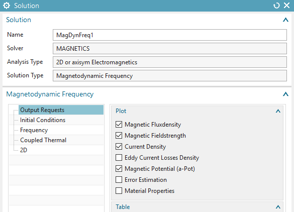
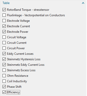
Some remarks to the requested outputs:
RotorBand Torque – stresstensor:
This is the usual result for the appearent torque in the air gap. It is
computed by the Maxwell Stresstensor method.
Electrode Current:
The resulting electric current on voltage loaded faces
(electrodes).
Electrode Power:
This result will compute voltage times electric current on all faces
with loads (complex multiplication). The real part of this result is the
active power and the imaginary part is the reactive power.
Eddy Current Losses:
This result will compute power losses that result from eddy currents and
ohmic resistance. Also lamination effects will be taken into
acount.
Steinmetz Hysteresis Loss:
Based on the material property Kh, the frequency and the magnetic
induction b this result computes losses on all parts with Kh>0 using
the Steinmetz formula.
Steinmetz Eddy Current Loss:
Similar as above, but using the material property Kc and the
corresponding Steinmetz formula. This result is alternative to the above
Eddy Current Losses.
Phase Shift:
This result computes the angle between electric current and voltage on
each load. This is also known as Power Factor.
Efficiency:
The Efficiency result computes output power divided by input power.
Output power is computed by the resulting torque times rotor speed.
Input power is computed by the active power on electrodes or
circuits.
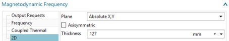
Set the thickness as shown in the ’2D’ options.
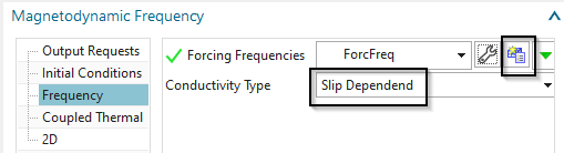
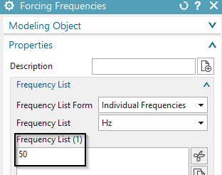
And the options for Frequency Domain: The forcing frequency
defines the velocity of the rotating field of the coils. 50 Hz divided
by the number of poles (4) gives defines
Hint: The Setting ’Conductivity Type’: ’Slip Dependent’ is basis for the
used induction motor analysis method.
Click Ok.
Switch to the FEM file
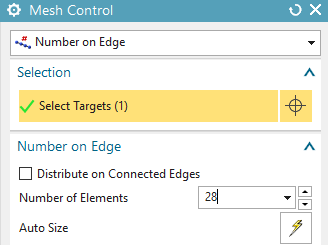
Create Mesh Controls ![]() :
:
Assign a number of 28 elements on the shown two linear
edges:
Assign a number of 20 elements on these two edges:
Assign a number of 180 elements on the two edges of the Moving
Band.

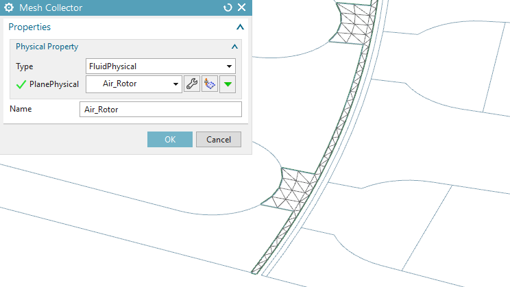
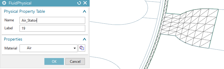
Mesh the inner part of the air gap (element size 0.5 mm). Create
a FluidPhysical and assign ’Air’ from the Magnetics material library as
shown in the picture.
Mesh the outer part of the air gap (0.5 mm) and also use
FluidPhysical and ’Air’.
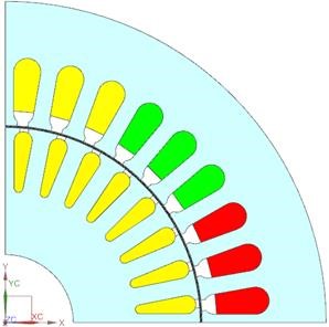
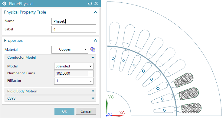
Mesh the coil faces (1 mm) for phase U and use the shown
settings.
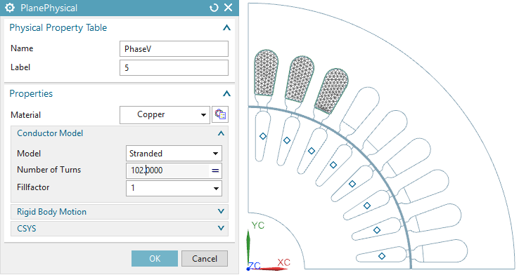
Mesh the coil faces for phase V and use these settings.
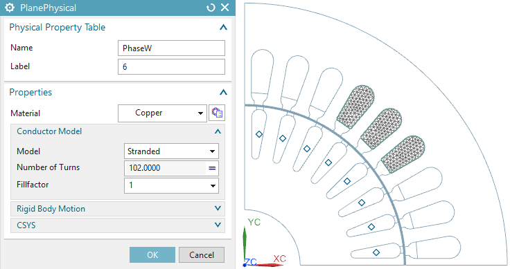
Mesh the coil faces for phase W and use these settings.
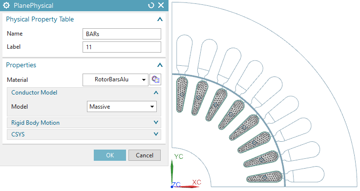
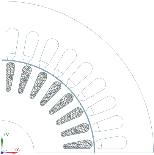
Mesh the bars (1 mm). Put them all in one physical or even in one
mesh. This will simulate the effect of connections at top and bottom.
So, in this case there is no need for an additional circuit network to
couple the bars. Use the shown settings. Create a new material for the
bars. Name it ’RotorBarsAlu’. Use the properties as shown and described
following.
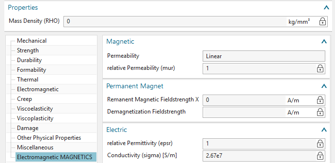
Some words about the properties of material Aluminum_Sample1:
Mass Density (RHO): 7.7e-6 Kg/mm3.
This property must be given if transient thermal is coupled with the
electromagnetic solution.
Electromagnetics: Relative Permeability (mur): 1
With mur = 1 the material has the same magnetic characteristic as
air.
Electromagnetics: Electric Conductivity (sigma) : 25380710
S/m.
This property is very important for induction effects. The appearance of
eddy currents strongly depends on this.
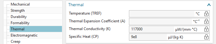
Thermal/Electrical: Thermal Conductivity (K): 117 W/m K
Basic characteristic for thermal conduction effects. This property must
be applied if thermal analysis is coupled with
electromagnetics.
Thermal/Electrical: Specific Heat (CP): 900 J/Kg K
The CP property is responsible for transient thermal effects. It must be
applied if any transient thermal is coupled with
electromagnetics.
The next picture shows the material dialog of
Aluminum_Sample1.
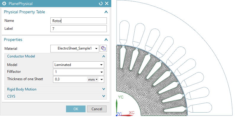
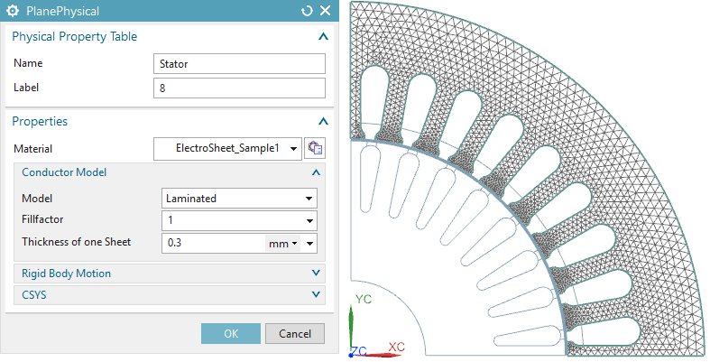
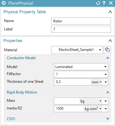
Mesh the rotor (1 mm) and use the shown settings. Use the library
material ’ElectroSheet_Sample1’ from the Magnetics library. Notice the
setting of the ’Conductor Model’. The ’Laminated’ model simulates the
behaviour of eddy currents and the corresponding magnetic field in thin
laminated sheets. The larger the value for ’Thickness of one Sheet’ the
more eddy currents and losses will appear.
Some words about the used material properties in ’ElectroSheet_Sample1’:
Mass Density (RHO): Needed only for transient thermal effects.
Electromagnetics: Relative Magnetic Permeability (mur):
1500
This property is used in case of frequency domain analysis or if there
is no BH curve given.
Electromagnetics: Electric Conductivity (sigma): 5800000 S/m
Electromagnetics: Core Loss Hysteresis Coefficient (Kh): 650
\(W/m^{3}\).
This value must be given by measurements or by the material
supplier.
Electromagnetics: Core Loss Eddy Current Coefficient (Kc): \(1.2 W/m^{3}\).
This value can be found by test simulations or is also given by the
material supplier.
Thermal: Thermal Conductivity (K): 35 W/m C
Thermal: Specific Heat (CP): 460 J/Kg K
Mesh the stator (2 mm) and use these settings:
All necessary work in the Fem file is done. Switch the displayed part to the Sim file.
In this section we will use a frequency domain solution to find motor characteristics at one operating point or rotor speed.
Create a simulation object ’Enforced Motion 2D Frequency’:
Select the ’Airgap Rotor Edge’ and ’Airgap Stator Edge’.
As a preparation for the following parameter sweep, instead of using a fixed value for the ’Angular Velocity’, you may easily create an expression named ’vel’ and couple this with the value of 800 rev/min. You do this by simply writing vel=800 into the ’Angular Velocity’ field. Later this expression can be used in a parameter sweep.
Key in 4 in the field ’Number of Poles Total’.
Select ’Air’ in the material field in box ’Airgap, auto
meshed’.
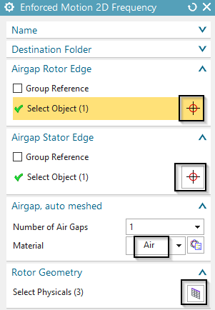
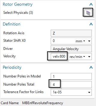

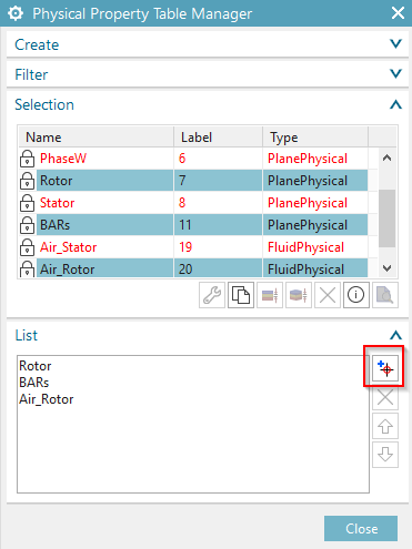
In ’Rotor Geometry’ select the three Rotor Parts, hit the ’Add’
button and ’Close’.
Click OK and the simulation object is created.
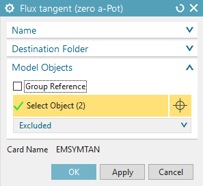
Create a constraint of type ’Zero Potential – Flux tangent’ on
the two boundary faces:
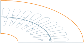
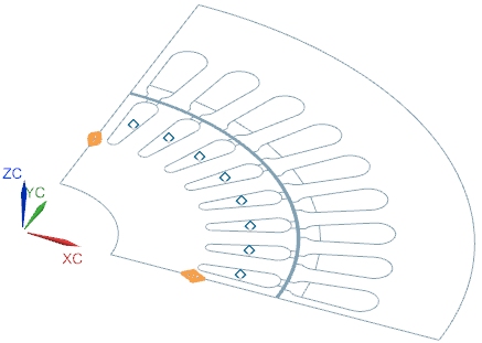
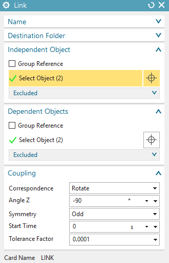
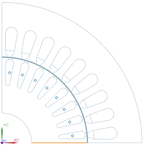
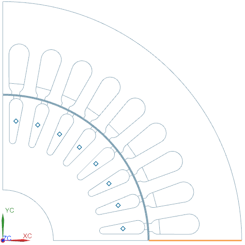
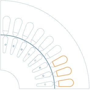
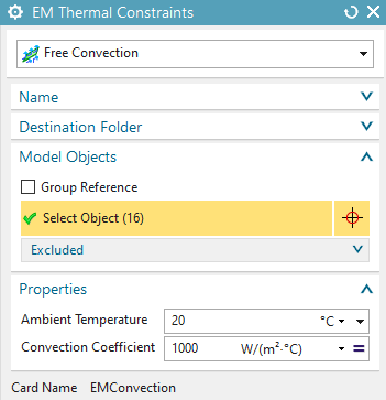
For periodicity conditions create two constraints of type ’Link’.
The selection should be done in mathematical positive direction, e.g.
against the clock sense. So the ’Independent Object’ must be the
highlighted (orange) edge in the next picture. The ’Dependent Object’
will then be the corresponding edge (vertical), rotated about 90 degrees
in positive direction. Use the settings as shown. Select also the small
edges of the air gap.
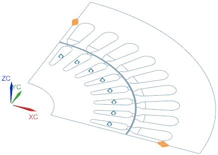
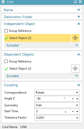
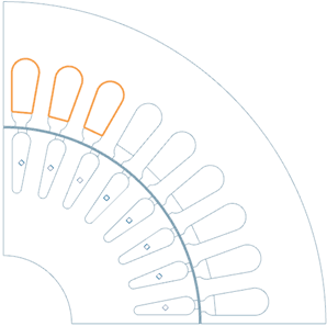
Create a second Link constraint for the edges of the
stator:
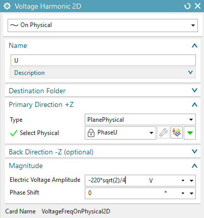
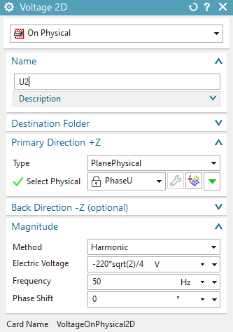
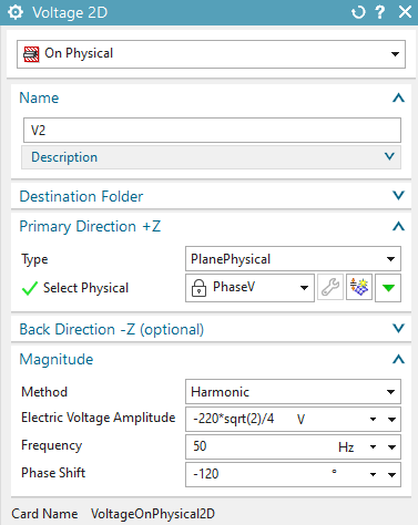
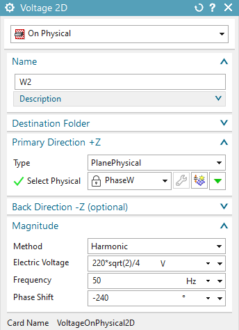
Create the following ’Voltage Harmonic 2D’ loads: Hint: We apply only 1/4th of the full voltage load because the model contains only 1/4th of the full motor. So the formula we use for the voltage is: 220 V * sqrt(2) /4 . Here 220 is the effective voltage. Don’t forget the phase shifts in the following three dialogs.
For phase U:
For phase V (phase shift -120):

For phase W (positive value, phase shift -240):


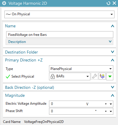
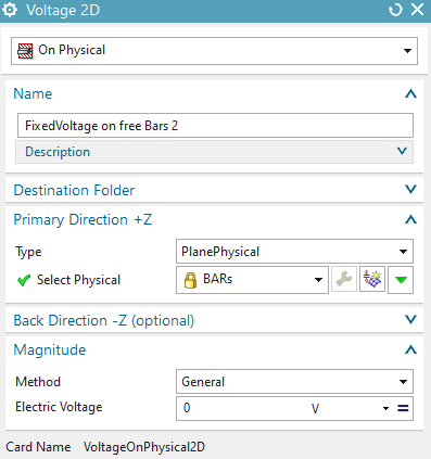
Create one additional voltage load on the rotor bars. Name this
load ’FixedVoltage on free Bars’ and apply zero voltage.
Solve the solution.
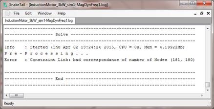
Hints: In some cases there may appear an error message (see picture)
saying that one of the link constraints didn’t find its corresponding
nodes. This message tells you that there are different numbers of nodes
on both edges. You can fix this problem by adjusting (probably one
element more or one less) the mesh control on one of the edges.
The solution will give the result for an operating point with 800 rev/min. To find results for other velocities change the velocity in the motion joint and solve again or run a parameter sweep as shown in the next section ’Sweep over Rotor Speed’.
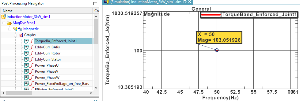
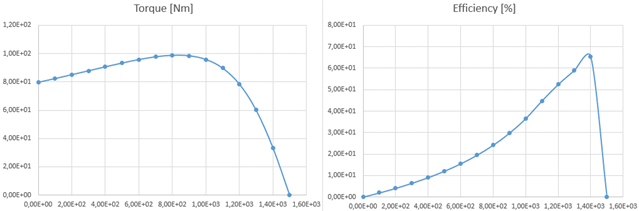
The resulting torque is 103 Nm. It can be found in the Post
Processing Navigator at ’Graphs’, see picture below.
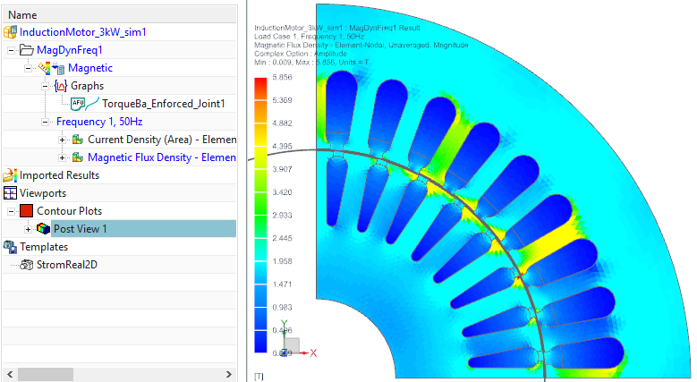
Magnetic Flux Density (also called ’Induction’): Use the ‘Set Result’ button to choose between Amplitude, Phase or Real and Imaginary part.
Hints to complex results: Because this is a frequency domain
solution, all loads and results are assumed to be harmonic. Therefore
all results are complex, described by real and imaginary parts.
Amplitude results (the geometric addition of real and imaginary part)
represent the peak values of such harmonics. Other interesting results
can also be extracted from the complex results.
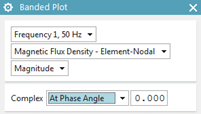
To study animations over time set the option ’Complex’ to ’At
Phase Angle’ and run the ’Animation’.


The Vectorpotential z direction result: (left: Real part, right:
Imaginary part). This result shows the magnetic field lines.
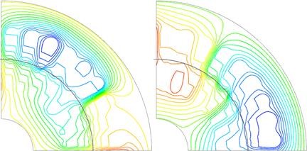
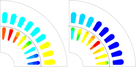
The Current Density result: (left: Real part, right: Imaginary
part)
Now we will use a parameter sweep to step over the whole speed range. By this way we will find the characteristic curves describing the motor.
Clone the Solution ‘MagDynFreq1’ and rename the Clone ‘MagDynFreq1_Sweep’. Open the ’Solver Parameters’ of solution MagDynFreq1_Sweep and change to register ‘Par.Sweep, SolveAgain’.
Set the ‘Perform’ option to ‘One Parameter Sweep’ and set the
settings as shown.
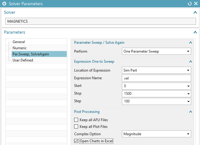
Some words about the settings:
Accept the default ’Location’ for the expression: ’Sim Part’ because the expression ’vel’ resides in the Sim part.
Expression Name: This must be an existing expression. To check for expressions you can use Tools, Expressions.
Start, Stop and Step: This defines the sequence of simulation steps.
’Complec Option’: This setting allows the selection or either ’Magnitude’ or the real, im parts of the complex result.
’Open Charts in Excel’: The parameter sweep results will be written into a vbscript file that can be pushed to MS Excel. Excel must be installed on the computer for that.
Solve the solution. Notice the progress bar at the bottom of the
NX window. It shows the percentage progress of the steps. Also notice
the vbscript (vbs) file in the working folder. It contains all requested
tabular results.
After solve has finished Excel starts and shows the requested results as curves over the given parameter.
Torque and Efficiency over speed:
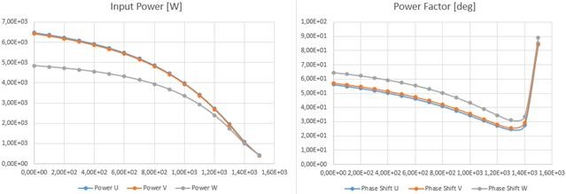
Input Power and Phase Shift (Power Factor) over speed:
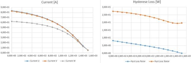
Current and Hysteresis Loss over speed. Be aware that the
computed hysteresis loss in frequency domain is not very accurate,
because only one frequency is taken into consideration. The later time
domain analysis will show higher hysteresis losses.
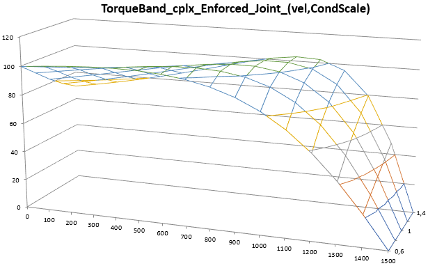
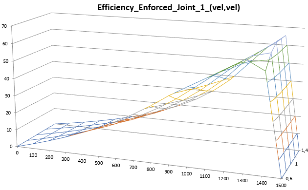
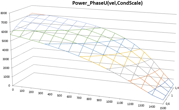
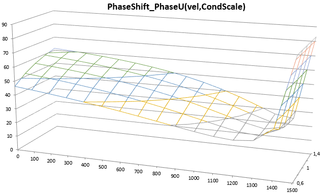
In many cases it is of interest sweeping over two parameters. For this motor we want to know for instance how torque and efficiency changes with the speed but also with the electric conductivity of the bars. The result will be shown as a surface graph in excel.
Clone the Solution ‘MagDynFreq1_Sweep’ and rename the Clone ‘MagDynFreq1_TwoSweep’. Open the ’Solver Parameters’ of solution MagDynFreq_Sweep and change to register ‘Par.Sweep, SolveAgain’.
Set the ‘Perform’ option to ‘Two Parameters Sweep’ and set the
settings as shown. There will be a parameter ’CondScale’ in the Fem
part. This parameter will scale the conductivity of the bars.

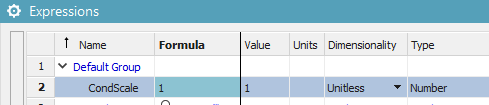
Change to the Fem part and create an expression (shortcut
Strg+e). Name this ’CondScale’ and set it to ’Unitless’.
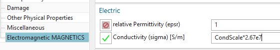
Edit the material properties of the bars and key in
’CondScale*2.67e7’ for the electric conductivity.
Change the displayed part to the Sim file and solve the new solution. The resulting graphs will look as shown below.
Torque and Efficiency over speed and bar conductivity:
Input Power and Phase Shift (Power Factor) over speed and bar
conductivity:
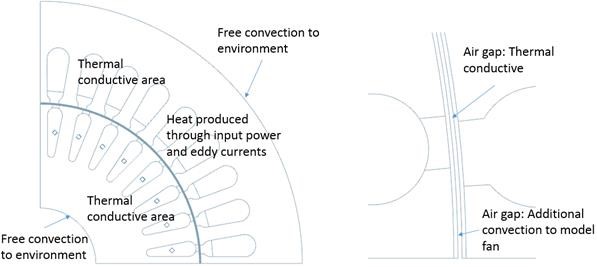
In this section, we will include simple 2D thermal analysis methods
for the induction motor. In more detailed simulations this must be done
in 3D to capture end effects and the motor housing. In this example, we
will directly use the power losses from the electromagnetic analysis as
input loads for a thermal solve. We include the effects of thermal
conduction in all parts. Also, we include thermal convection effects
with given fixed coefficients to model water cooling. The air gap is
modeled as a thermal conductive area, so heat produced in the rotor can
travel through the air gap into the stator. To capture the effect of
cooling by a fan we add additional convection to the air gap.
In this case we use a set of given convection coefficients. Of course,
these values strongly influence the thermal results of the simulation.
To find realistic values for convection coefficients simulations should
be calibrated with experiments. Another way to find values is through
analytical considerations by use of convection formulas that model shear
flow between two moving plates. Such formulas can be found in standard
literature like ’VDI Wärmeatlas’.
We first run an analysis at one operating point and afterwards a sweep
over the full range. We choose a speed of 1400 rev/min because of its
best efficiency as we have found in the previous section. Since the
material properties already have all information for this thermal
analysis we can continue with solution settings. Remember the necessary
material data that is needed for this is only Thermal Conductivity (K).
In case of transient analysis the Thermal Capacity (CP) would be
needed.
Clone the solution MagDynFreq1_Sweep and rename it to MagDynFreq1_Thermal_Sweep.
First switch off the parameter sweep (in ’Solver Parameters’). We will activate it later.
Edit the expression vel and set it to 1400 rev/min (Tools, Expressions …).
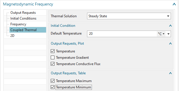
Edit the solution and change to register Coupled Thermal.
Change the Thermal Solution to Steady State. This will compute the settled thermal situation while running at the given operating point.
Activate the Output Requests as shown.
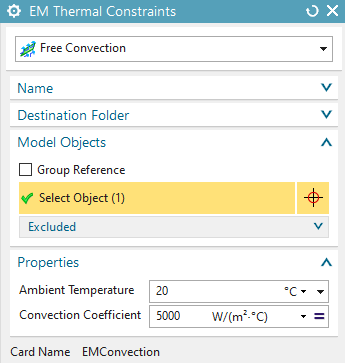
We want to model the effect of a water cooled outside stator face.
Create a constraint of type ’EM Thermal Constraints’ and set the Type to ’Free Convection’.
Select outside edge.
Key in the values as shown below. Notice the unit of the
convection coefficient: W/m2 C.
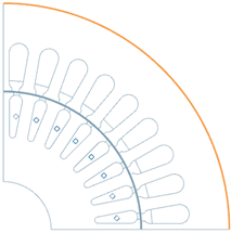
Similar we model a cooling inside the rotor with smaller coefficient.
Create a constraint of type EM Thermal Constraints and set the Type to Free Convection.
Select inside edge.
Key in the values as shown below
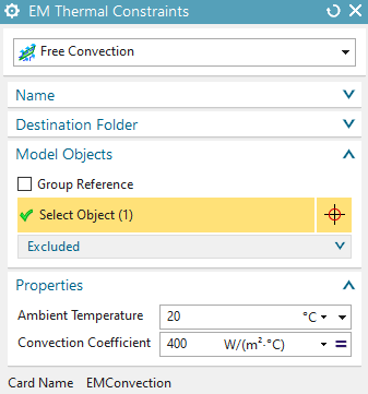

Next create a Free Convection constraint on the rotor edges. This
will simulate the effect of cooling air from a fan flowing through the
air gap.
Switch off the parameter sweep (if not already done) and solve the solution.
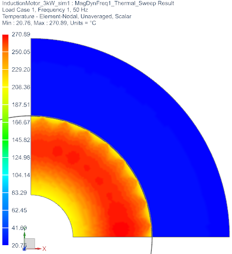
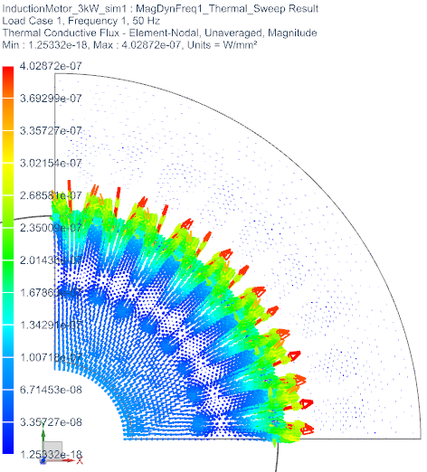
The resulting temperature field at 1400 rev/min has a maximum
value of 270 C as shown in the next picture (left side). On the right
side, there is the thermal conductive flux displayed with vectors. The
thermal flux result helps understanding how the thermal energy is
produced and how it moves.
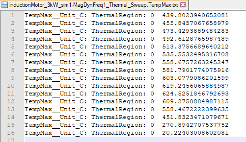
Activate the one parameter sweep. Because in this software
version the thermal sweep results are not written to the excel file we
must view them in text file. Therefore we set the solver parameter
’Result Tables (txt)’ to ’Append’. Solve the solution. After finish
there appear two additional results (maximum and minimum temperature) as
text files.
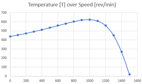
In an excel graph this gives the information about how
temperature behaves over the speed range:
Now we do a precise solve for the detailed computation of losses. Because of the transient solution it is possible also to accurately compute a nonlinear BH curve. Because of simplicity reasons we don’t use nonlinear material for this and we also don’t analyse for temperature. We choose 1400 rev/min as operating point.
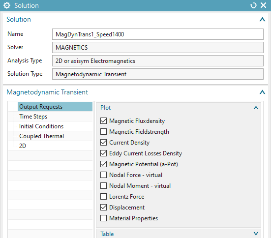
Create a new solution of type 2D Magnetodynamic, Transient. Rename the solution ’MagDynTime1_Speed1400’.
Set the Output Requests as shown.
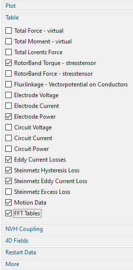
Some words to table results:
Motion Data: This option writes out the displacement step and total displacement of the motion joint at each time step. That is quite important, because it allowes creating graphs over the rotation angle.
FFT Tables: This option enables the fourier transformation of the active table results. In box More there are some options about the fourier transformation process but the defaults are good for now.
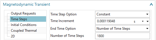
In register Time Steps:
Set the Time Increment to 0.000119048 sec. With a rotor speed of 1400 rev/min this corresponds to 1 degree per time step.
Set the Number of Time Steps to 1800. This corresponds to 5 times
360. So we will analyze 5 rotor turns. This should be enough to decay
the transient that we expect due to sudden start.
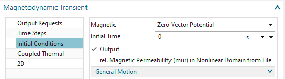
In register ‘Initial Conditions’: Set the ‘Magnetic’ option to
‘Zero Vector Potential’. This is the best starting condition for this
voltage driven system.
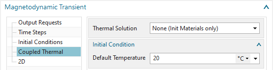
In register ‘Coupled Thermal’: Use the default option None.
Because this simulation will cover only a short time period there are no
meaningful thermal results expected.
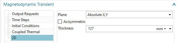
In register ’2D’: Key in the thickness.
Drag all but the thermal constraints into the new solution. You
can simply reuse the existing ones.
The loads must be created newly because they are different from
the frequency solution loads. Create 3 new loads on the corresponding
coil faces. Use type ‘Voltage 2D’, Type ’on Physical’ with Method
‘Harmonic’. Take care of the correct signs of the values (see picture
below).
Also the load with zero voltage on the Bars must be newly
created.
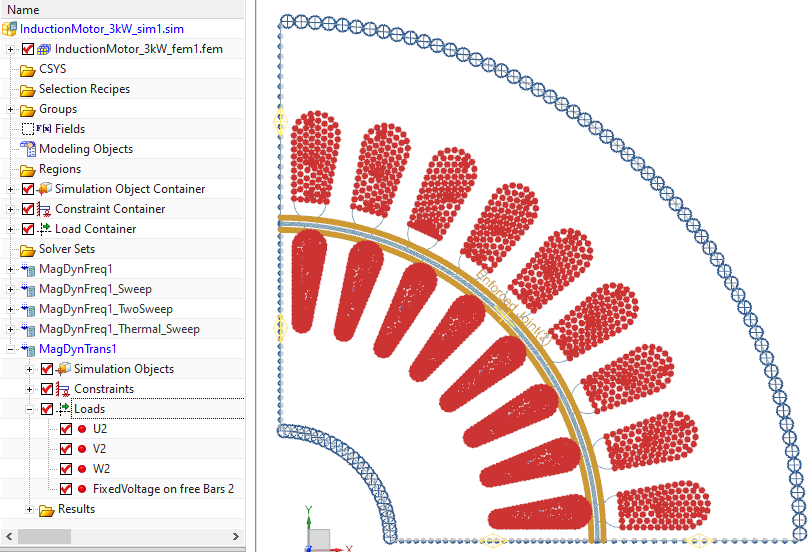
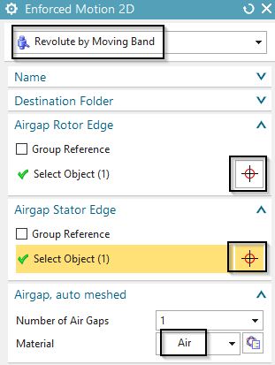
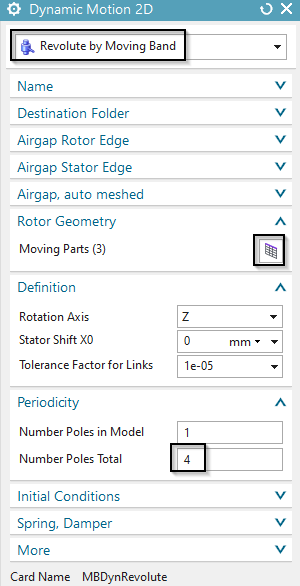
Create a ‘Simulation Object’ of type ‘Enforced Motion 2D’. Accept the default type ‘Revolute by Moving Band’.
Select the Rotor and Stator Edges,
At ’Airgap, auto meshed’, choose ’Air’,
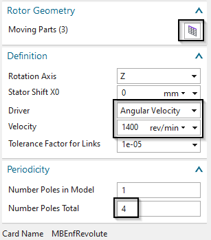
For ’Rotor Geometry’, select the physicals Rotor, BARs, AirRotor.
Set the ’Driver’ to ’Angular Velocity’,
Key in ’Velocity’, ’Number of Poles total’ (see picture below).
Click OK to finish the dialogue.

Solve the solution. Because of the number of steps the solve process will take about 10 - 15 minutes.
After the solution has finished check the tabular results.
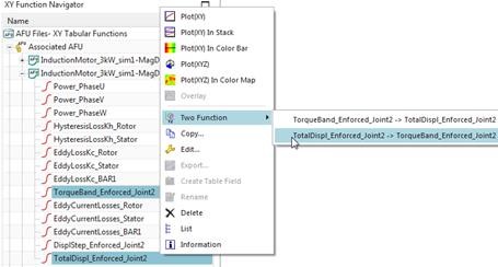
Hint: By default the AFU graphs show time on the abscissa.
Instead you can set the rotor angle (or any other result) to the
abscissa using the following method: Select in the XY Navigator two
curves, Torque and TotalDispl. Then choose RMB Two Function and choose
the second from the two possibilities (see picture).
The Torque result shows transient behaviour at the beginning and
becomes more and more stationary after time.
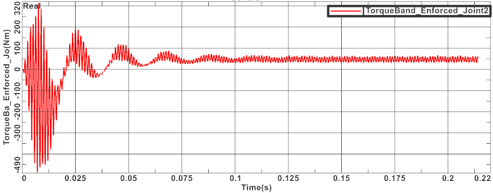
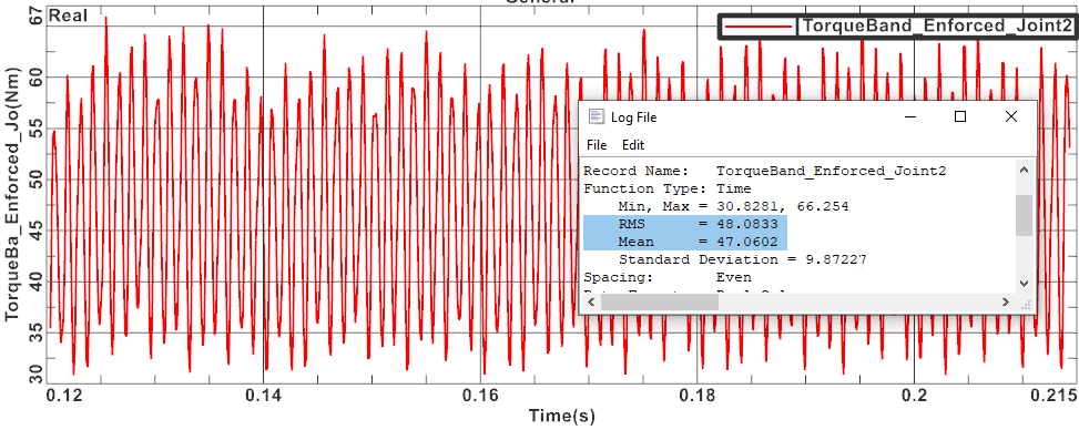
Let’s compare this to the torque we found with the prior
frequency domain analysis: There we had 47.7 Nm at 1400 rev/min. Here,
if we cut the transient as in picture below, there appears an
oscillation between about 30 and 60 Nm with RMS 48 Nm. So, both time and
frequency results are very near. The time domain analysis is more
precise and additionally it captures torque ripple information.
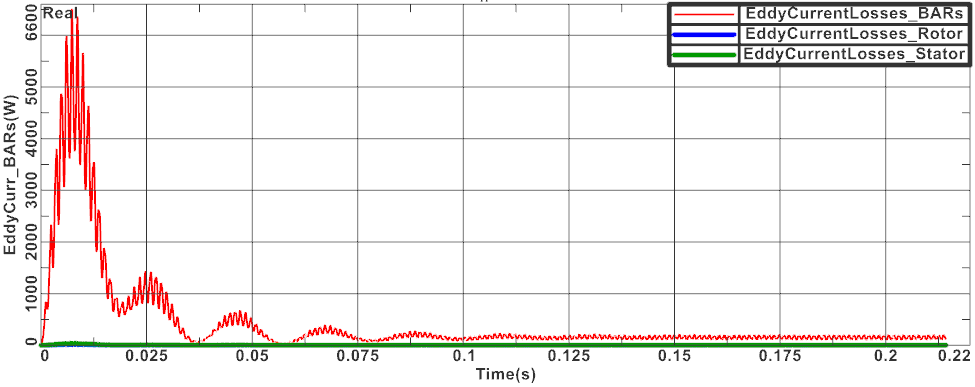
The Eddy Current losses on bars, rotor and stator also shows the
transient, mainly on the bars. Other results, like power on the thress
phases are also available.
The Hysteresis Losses on Rotor and Stator are computed after all
time steps have finished. This additional post processing step can
consume much time. For the computation Fourier transformations are
performed at each element to find dominant frequencies and amplitudes.
By default the system computes 15 frequencies. Let’s compare again these
values to those from the frequency domain analysis: in time domain, we
find 77 watt on the stator and 5.6 watt on the rotor. The frequency
analysis showed much smaller values and is less precise, because it
takes into account only the first, dominant frequency.

It is also of interest to analyse the transient start behaviour of an induction motor. To do so we have already applied nearly all information. Two things are missing: The mass inertia property of the rotor and a dynamic joint instead of the enforced one.
Change to the Fem part and edit the physical properties of the
rotor. Key in the value 1500 Kg mm2 for Inertia RZ. This value can be
found by running the CAD function Analysis, Measure Body ![]() using the detailed CAD geometry and mass density information applied to
the rotor.
using the detailed CAD geometry and mass density information applied to
the rotor.
Change to the Sim file again and
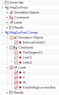
Clone the solution ‘MagDynTime1’ and rename the new one to ‘MagDynTime2_MotorStart’.
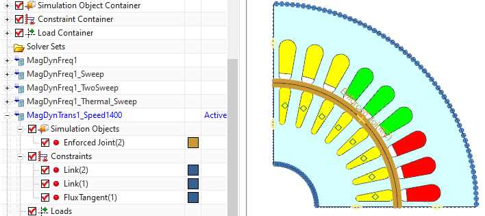
Remove the Simulation Object ‘Enforced Joint’ from the new solution.
Create a new Simulation object of Type ‘Dynamic Motion 2D’ (see picture above right). Select Rotor and Stator Edge, key in ‘Number of Poles’ and ’Rotor Geometry’ same way as before.
Modify the voltage load to 50 percent.
Solve the solution. Again it takes 10 – 15 minutes.
After solving you can display the following graphs:
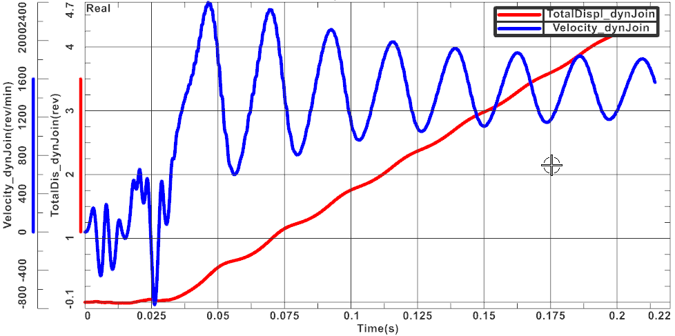
Total angular displacement (red curve) and Velocity (blue curve)
over time (set the units to rev and rev/min). It can be seen that after
the transient there appears still oscillation but the velocity reaches
more and more the synchronous value of 1500 rev/min.
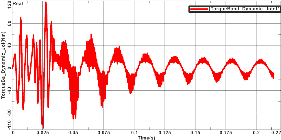
Torque over time. The torque becomes smaller the more we reach
synchronous speed.
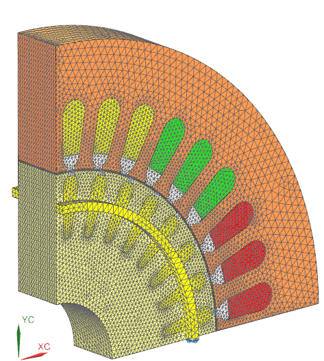
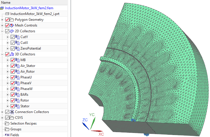
In the complete folder of the tutorial there is also a 3D model of
the motor that is set up pretty much the same as the 2D model from the
beginning. This 3D model would additionally allow to study end effects
and other 3D specific effects. The thickness is reduced to 12.7 mm. So,
if results shall be compared to the 2D model, this must be set to the
same thickness. All used features can be found in the model files.
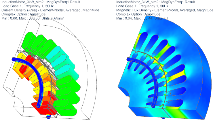
Open the file ’InductionMotor_3kW_sim2.sim’ from folder ’complete’.
First check the solution ’MagDynFreq1’. It is from type ’Magnetdynamic Frequency’ with 50Hz. For ’Output Requests’ we are interested in the RotorBand-Torque, the ’Current Density’ and the ’Magnetic Fluxdensity’.
Switch to the fem file.
Notice that there are three 2D mesh collectors. The ’CutY’ and the ’CutX’ collector, that contain the meshes of the cutted faces and the ’ZeroPotential’ collector.
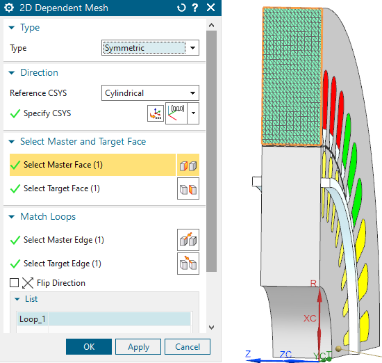
Open the ’CutY’ collector to see the meshes. Every ’CutY’ mesh has a corresponding mesh in the ’CutX’ collector. Those are createtd by the ’2D Dependend’ feature.
Click ’Edit’ on ’CutX4’ to see the settings of this mesh. For
’Master Face’ the upper face is selected, the program automatically
selects the corresonding ’Target Face’ on the other side of the motor.
It also selects the ’Master’ and Target Edges’. It is important, that
the arrows of the ’Master’ and ’Target Edge’ point in the same
direction.
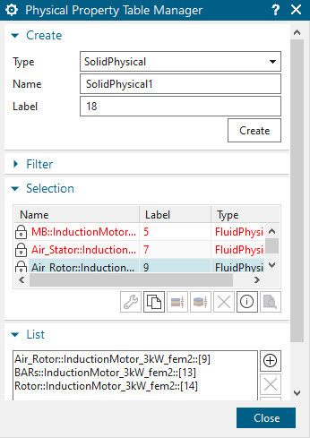
Check the 3D collectors. We use the same physical properties as in the 2D simulation.
Now switch to the sim file.
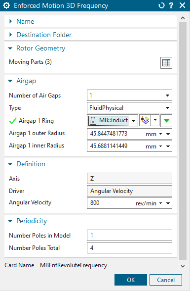
Check the ’Simulation Object’ in the solution.
It is from type ’Enforced Motion 3D Frequency’, for ’Moving Parts’ the ’Rotor Air’, the ’Bars’ and the ’Rotor’ are selected.
For ’Airgap 1 Ring’ the ’Moving Band’ is selected, and the
’Angular Velocity’ is set to 800 rev/min.
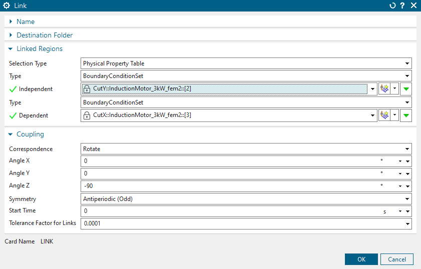
Check the Constaint, ’Link(1)’. For ’Independent’ the ’CutY’
physical is selected, for ’Dependent’ the ’CutX’. The ’Coupling’ is
simular to the 2D link.
Open the ’Loads’.
Now have a look at the loads. Load ’U’, ’V’ and ’W’ are shifted by \(-120^\circ\). They have a amplitude of 77.7817 V.
Now solve the solution.
Open the AFU-Graph of the ’RotorTorque_Enforced’.
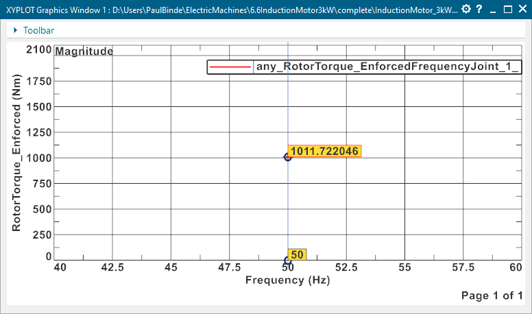
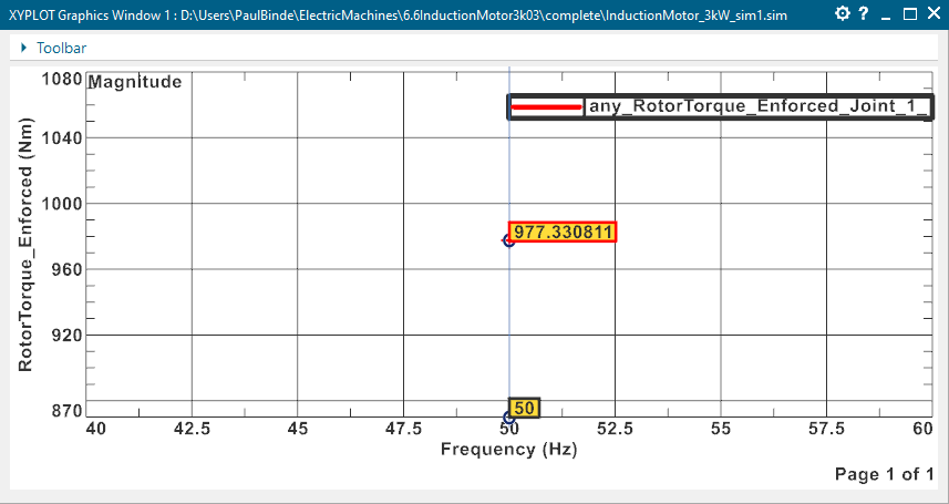
To compare this picture shows the torque of the 2D model with the
same thickness. The torque has almost the same value.
The tutorial is complete.