 Advantages of this method are
This tutorial shows how to model electric motors using the NX
assembly fem method. This method allows to create meshes only for parts
of the whole motor and then use those meshes multiple times in an
assembly (AFEM). The next picture shows this situation: The file
Stator_fem1.fem is created only once, but used several times in the AFEM
file Motor_asm_assyfem1.afm.
Advantages of this method are
The overall mesh becomes perfectly regular because the same mesh is used for each segment. Because of this there will also be more precise results.
Less meshing effort
Less data volume
You can find the already completed model of the simple motor in this tutorial folder. Go through the following steps to become familiar with the main features:
Download the model files for this tutorial from the following
link:
https://www.magnetics.de/downloads/Tutorials/6.CouplMotion/6.5ElectricMotorAFEM.zip
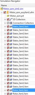
Open the file Motor_asm_sim1.sim.
Make the CAD assembly part Motor_asm.prt the displayed part.
Check in the assembly navigator the structure of this CAD
assembly. It contains one segment of the rotor and one of the
stator.
Change the window to the file Rotor_fem1.fem. Check the contents
of this file.
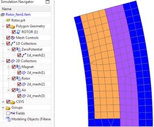
There is a 1D mesh at the outer border. This is applied to a Physical of type ZeroPotential. Therefore no additional constraint of this type is necessary anymore in the Sim file.
The Magnet has permanent magnet material and a cylindrical coordinate system as usual. Later in the Sim file we will see that every second magnet physical is overwritten and because of the need for opposing magnet directions.
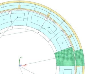
Change the window to the file Stator_fem1.fem. Check the contents
of this file.
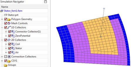
Again there is a 1D mesh at the inner border with Physical of type ZeroPotential. Therefore no additional constraint of this type is necessary anymore in the Sim file.
There is a 1D Connector mesh. This is later used to implement the network. The advantage is that this Connector must only be created once.
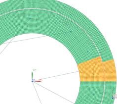
Change the window to the file Motor_asm_assyfem1.afm. Check the
contents of this file
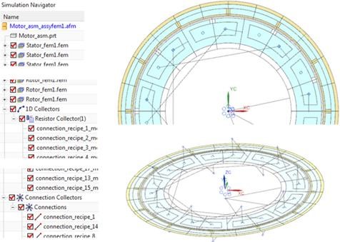
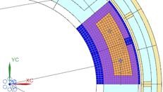
Notice that there are 18 Stator_fem1.fem files included in the
assembly fem file. For best exploitation of symmetry every second of
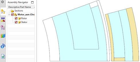
those meshes is positioned upside down. This method has the advantage of
perfectly matching nodes at borders. Next picture shows such a couple of
two meshes.
Notice the 1D resistor elements. They form the circuit network to couple the coil connectors.
Although nodes at borders are perfectly matching, they must be merged. In this model nodes are already merged, but in a new model you must check for duplicate nodes using the function Duplicate Nodes .
Like always in NX assembly fem you must use the Assembly Label Manager to resolve conflicts in labeling. Simply press ‘Automatically Resolve’ in the Assembly Label Manager.
Change the window to the Sim file Motor_asm_sim1.sim. Check the contents of this file.
Check the solutions in the Sim file. There is one static and one transient solution included. Loads and simulation objects are set up in the same way as without assembly fem. There is nothing special for afems now anymore.
The tutorial is complete.