In this example we show the usage of the ’Dynamic General Motion’
technique in the context of a 3D Relay.
Estimated time: 1 h
Follow the steps:
This example is shown using 3D, but the technique is possible in 2D very
similar. The corresponding model in 2D is stored at the same folder
location, so it can be seen there how it is set up.
Estimated time: 1 h
Follow the steps to reproduce it:
Download the model files for this tutorial from the following
link:
https://www.magnetics.de/downloads/Tutorials/6.CouplMotion/6.3Relay.zip
Open the part file ’relay3D.prt’.
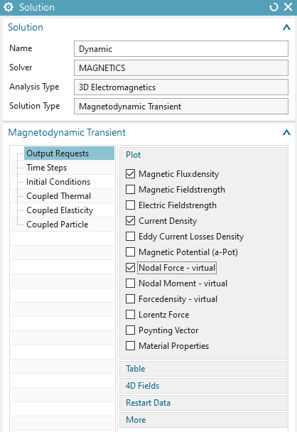
Start Simcenter Pre/Post, create a new Fem and Sim File for 3D.
Switch off ’Create Idealized File’,
Chose Solver ’MAGNETICS’ and Analysis Type ’3D Electromagnetics’,
Choose Analysis Type ’Magnetodynamic Transient’.
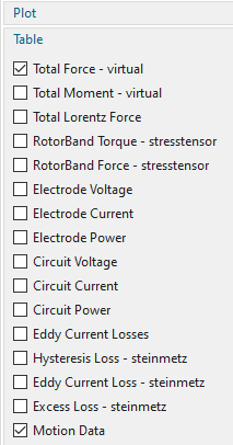
In register ’Output Requests’, ’Table’, activate ’Motion Data’.
Others can be activated as desired.
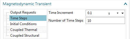
In register ’Time Steps’, select a time increment of 0.1 sec and
10 time steps.
Change to the Fem file.
In the following steps we create all 3D Meshes (all but the air gap). This will be done by tetrahedral elements and appropriate mesh collectors.
First, create mesh mating conditions. So, make all polygon bodies
visible, click on ’Mesh mating Condition’ ![]() , drag a window over the geometry, set the ’Mesh Mating
Type’ to ’Glue-Coincident’ (default), click ’OK’. Check, there will be
22 mesh matings created.
, drag a window over the geometry, set the ’Mesh Mating
Type’ to ’Glue-Coincident’ (default), click ’OK’. Check, there will be
22 mesh matings created.
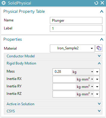
Then, mesh the Plunger with one fourth of the suggested mesh
size. Assign the material ’Iron_Sample2’ as well as a ’Rigid Body
Motion’ mass of 0.28 Kg.
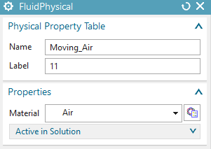
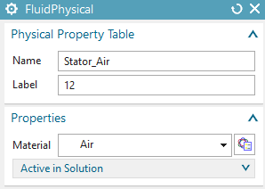
Mesh the (two) moving air stripes with one fourth of the
suggested element size. Use a ’FluidPhysical’ and assign material
’Air’.
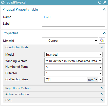
Mesh the first Coil with the suggested mesh size and assign
material ’Copper’. Also, set the ’Conductor Model’ to ’Stranded’ with 50
turns, a fill factor of 1 and a coil section area of 741 \(mm^{2}\).
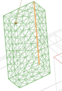
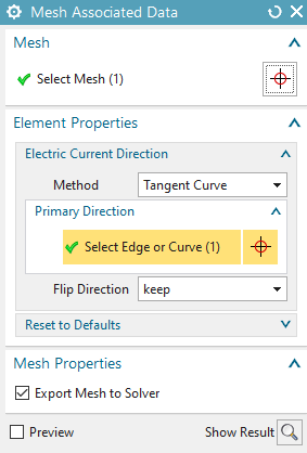
Edit the ’Mesh Associated Data’ of the coil mesh and define the
direction of current (use one of the z-dir edges. Take care that the
polygon body is shown.).
Proceed in the same fashion with the other three coils (meshing,
material and current direction).
Finally, create a mesh with one third of the suggested mesh size
for the stator air and set the small feature tolerance to 2%. Again, use
the type ’FluidPhysical’ for this.
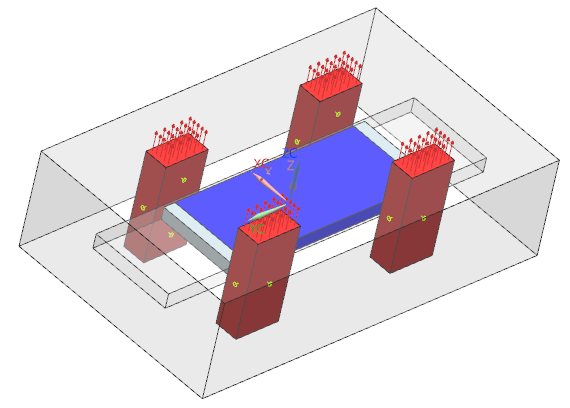
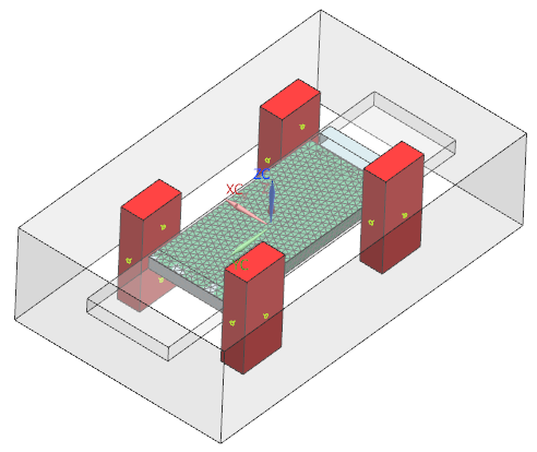
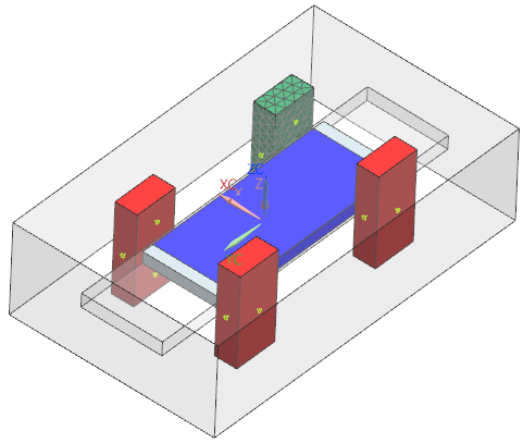
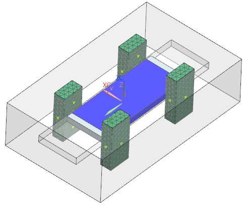
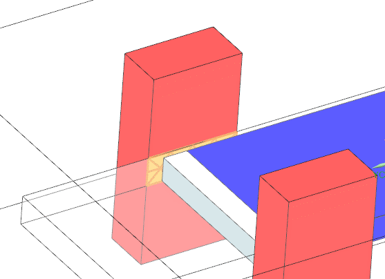
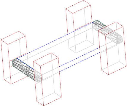
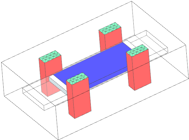
Following we do preparations for the 3D air gap mesh. E.g. the
mesh that will update with each movement step. Following picture shows
the plunger and how the updating air gap surrounds it. So, if the
plunger moves and the air gap is updated, a new simulation step can be
done.
This updating air gap mesh will be of type ’Solid from Shell Mesh’ and
therefore needs 2D boundary meshes from which it depends. Therefore, NX
Magnetics provides a feature that allows to recreate that mesh prior to
each solve. We will set up this feature now.
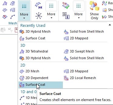
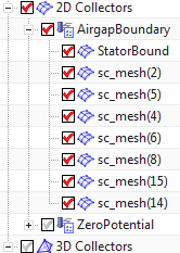
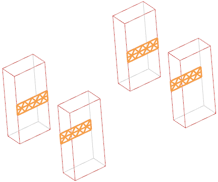
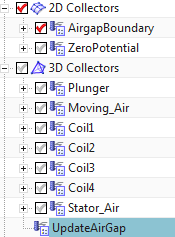
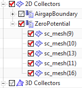
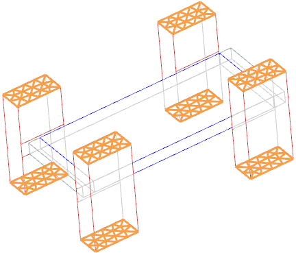
Following you create all boundary meshes of the updating air gap.
Therefore, you create surface coat meshes (picture below left) on all
faces that belong to the boundary of the air gap. The right side picture
below shows how the navigator looks after all the boundary meshes are
there.
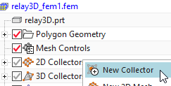
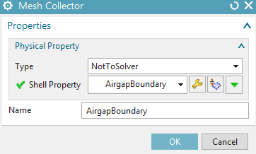
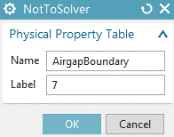
To collect the following meshes, first create an 2D mesh
collector, name it ’AirgapBoundary’. Use a physical of type
’NotToSolver’ because these meshes will act as borders only for the 3D
air gap mesh.
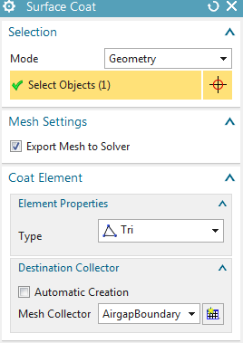
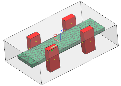
First, create a ’surface coat’ on the 4 inner side sections of
the four coils that are in contact with the moving air (see
below).
Next create surface coat meshes for the left (e.g. green mesh)
and the right surface parts of the moving air.
Then, create a surface coat mesh for the moving air.
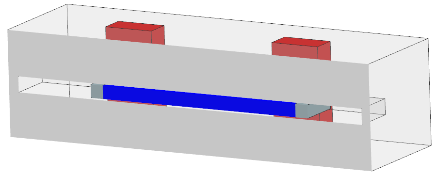
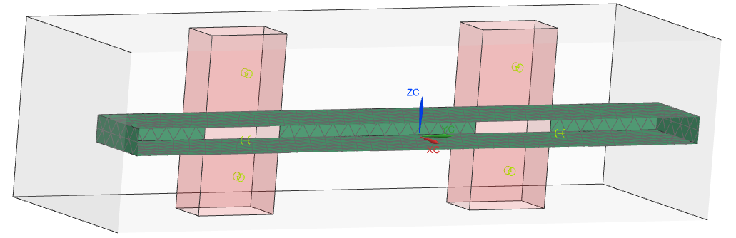
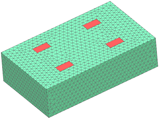
Finally, create a surface coat mesh stator bound air (that
provides the extend over which the air can move). For easier selection
of these interior faces of the ’Stator_Air’, use the helpful ’Clip
Section’ feature from toolbar ’View’. Select all inside faces of the air
as shown in the picture below (Note: You have to invert the clip section
to select the faces on the opposite side).
When all boundaries are visible, it should look like the
following picture.
With these air gap boundaries being completed we now set up the automatically updating 3D air gap mesh:
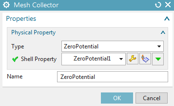
Create a 3D mesh collector.
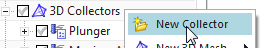
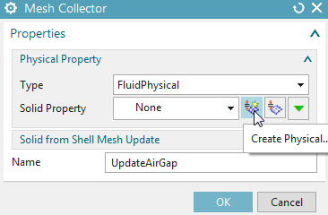
Name the collector UpdateAirGap, set the physical type to
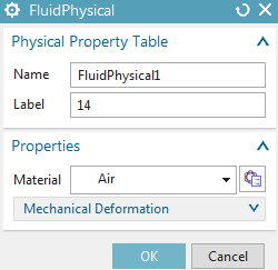
FluidPhysical, click Create Physical and set the material to Air. Click
Ok.
Back in the mesh collector dialogue expand the box ’Solid from
Shell Mesh Update’ and set the option Activate to ’Create/Update Mesh at
Solve’.
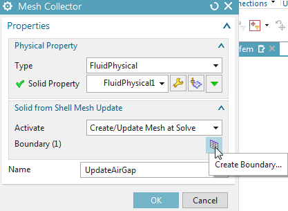
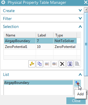
Click on ’Create Boundary’ and in the following dialogue select
the previously created physical AirgapBoundary that holds the 2D
boundary.
Click Close, Ok and the mesh collector is created. Notice that it contains all necessary information to create a Solid from Shell Mesh, but the mesh itself will be created at solve time. (Alternatively you can create the mesh manually now, it makes no difference).
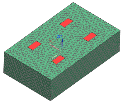
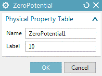
Now create all outer 2D surface coat meshes (equivalent as in the
last step). However, in contrast to the last step, use a physical
property of type ZeroPotential. Hint: We do this procedure in order to
fix the Boundary condition (i.e. ZeroPotential) directly in the .fem
file. However, this could also be done in a later step in the .sim
file.
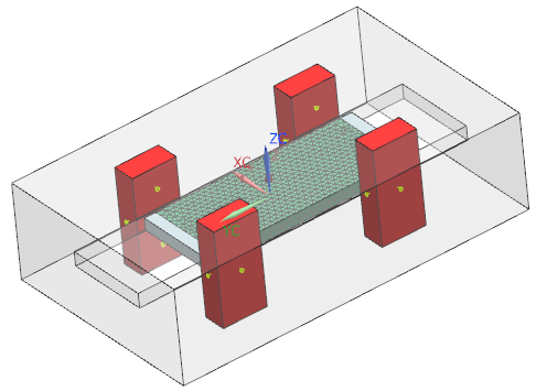
First, create surface coat meshes for the top and bottom sides of
all four coils (see picture).
Then create a surface coat mesh for the outer air.
Meshing is done, change to the Sim file.
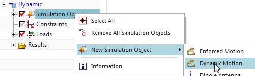
Create a Dynamic Motion to define the movement of the plunger.
Create a simulation object of type ’Dynamic Motion’. Activate
’Slider by General Motion’.
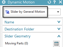
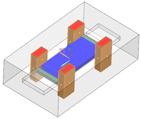
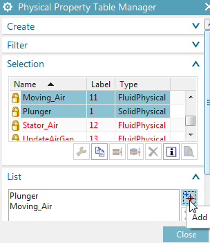
In the dialogue first define the Slider Geometry. Click on
’Create Moving Parts’ and add the two physicals Moving_Air and Plunger
that will move to the list. Click Close.
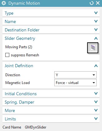
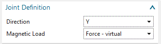
Back in the Dynamic Motion dialogue, set the Direction to Y and
accept all other defaults with Ok.
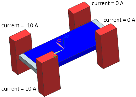
Define the electric currents on the four coils: Define zero
amperes on the two right coils (see picture) and define 10 and -10
amperes on the two left coils. This will result in a Y force on the
plunger.
Solve the solution.
Post processing.
We first check the motion data result. This contains Total Displacement, Displacement Step and Velocity.
Open the associated result file in the post processing navigator. A list of all tabular results appears above the plot results.
plot the three results as shown below.
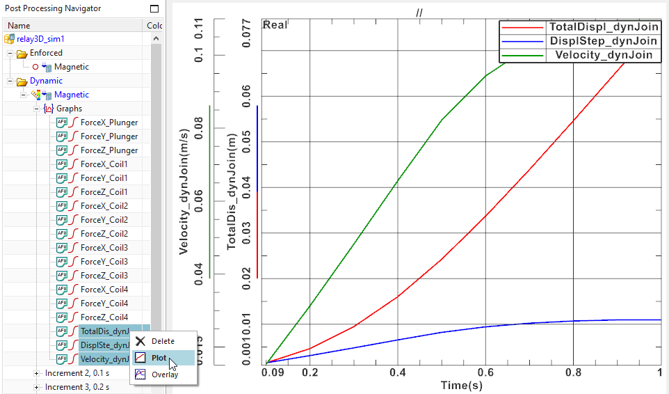
If acceleration is needed this can be derived by differentiation using the mathematical operations for afu graphs.
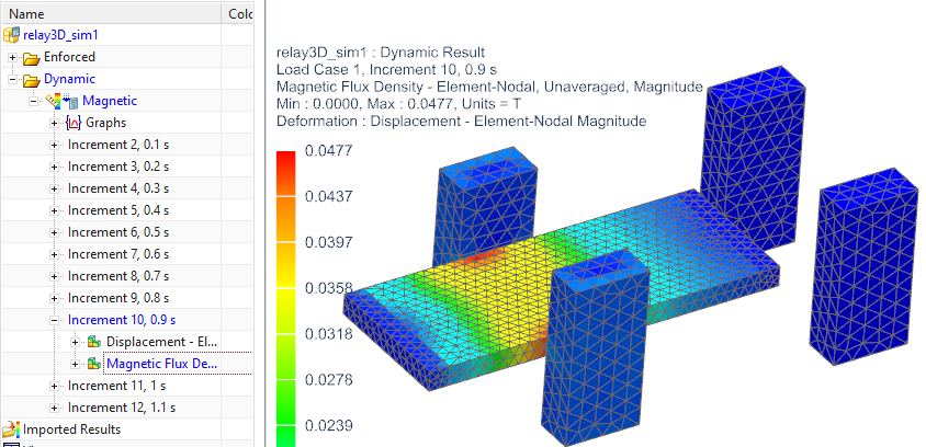
Next we check the plot results. After 10 time steps the Magnetic
Flux density field on the slider should look as follows
This ends the tutorial.