In this tutorial we analyse a rotor that is moving between two
permanent magnets. First we apply a forced speed of 5.000 turns per
minute and then we analyse the free motion behaviour.
Different techniques are shown here, so we use 2D as well as 3D
modeling. And we use two different motion techniques for rotation:
’General Motion’, a feature that can be used for 3D rotation and
translation. And the ’Moving Band’ technique, that is capable for 2D
rotation only. Also we show free (dynamic) motion as well as enforced
motion. Thus, the tutorial is split into four parts:
2D enforced,
2D dynamic,
3D enforced,
3D dynamic.
Two permanent magnets are positioned near the rotor. This leads to
time dependent variations of the magnetic field and therefore eddy
currents will appear in all electric conducting parts. In reality such
eddy losses will lead to temperature rise, an effect that is neglected
in this basic tutorial but could be simulated by a coupled thermal
solution. Those eddy currents shall be displayed and resulting power
loss shall be computed. The enforced analysis shall be done over 45
degrees, the dynamic one over a time period that allows observing the
expected oscillations. The CAD models of both the 2D and 3D base on the
same ’Skelett.prt’ file.
2D Enforced Driver
The following example a pure 2D example; and thus not designed to
work in 3D. In this example, an iron rotor rotates between two permanent
magnets. The example shows how to perform analysis’ that couple
electromagnetics and mechanical movement. In the present scenario the
motion is simulated with an enforced motion; however, it can also be
simulated with dynamic motion. This is done in the next tutorial. Then,
the movement would have one degree of freedom in the mechanical sense.
The example is executed in 2D because of the shorter solution time but
it would be similar in 3D as is shown in a further example.
Main goal is to model the enforced motion effect of the rotor. Other
results like eddy currents can be requested additionally if
desired.
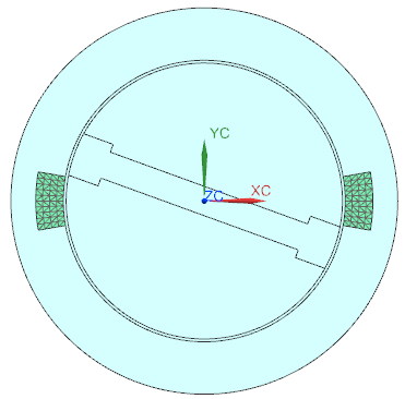
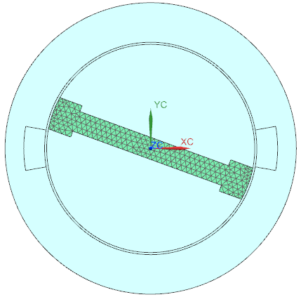
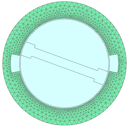
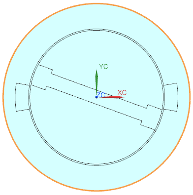
Here, the start position of the rotor is set to -20
degrees.
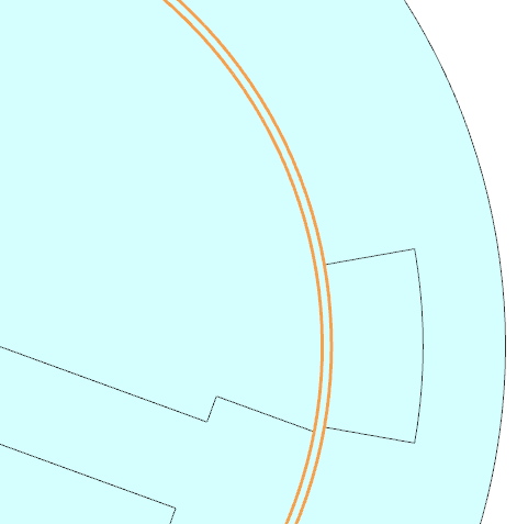
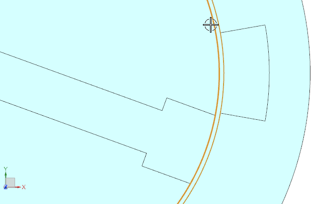
Also, there is a ’Moving Band’ visible. This has two circular
edges, one connected to the moving part and one to the stator regions.
At each time step the solver will rotate the moving regions and create a
mesh between the two edges automatically.
Start Simcenter Pre/Post, create a new Fem and Sim file for 2D
Electromagnetics.
Switch off ’Create Idealized File’,
Choose Solver ’MAGNETICS’ and Analysis Type ’2D or axisym
Electromagnetics’, OK,
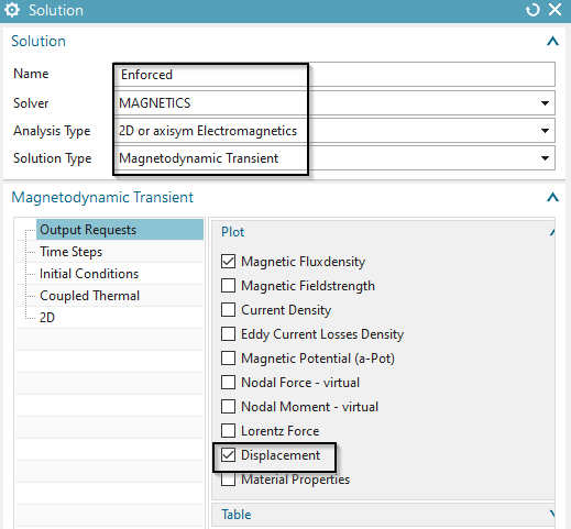
Set the ’Analysis Type’ to ’Magnetodynamic Transient’ and name
the solution ’Enforced’.
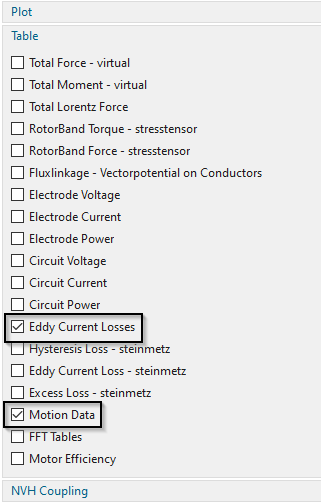
In register ’Output Requests’,’Table’ activate ’Motion Data’ and
in ’Plot’ activate ’Displacement’ as well as ’Magnetic Fluxdensity’.
Others can be activated if one is interested.
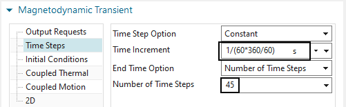
In register ’Time Steps’ set the ’Time Increment’ to
1/(60*360/60). This formula corresponds to a rotor speed of 60 rpm (1
rps).
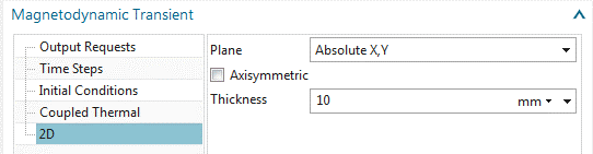
In register ’2D’ set the ’Thickness’ to 10 mm.
OK.
Switch to the Fem File.
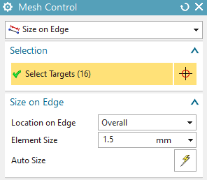
When using the Moving Band technique the band elements should
have about the same element size. Therefore, create a ’Mesh Control’
, use type ’Size on Edge’, select the outer and inner
edges of the moving band, set the ’Element Size’ to 1.5 mm and click
OK.
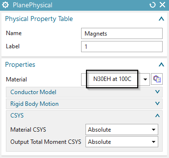
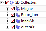
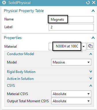
Create a Tri-Mesh on the Magnets. Use the suggested element size
and assign material ’N30EH at 100C’. The permanent direction of north is
X by default, so we can stay with the default for our example. Assign
the name ’Magnets’.
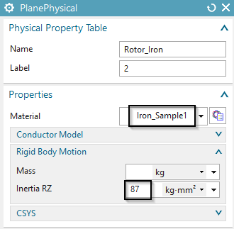
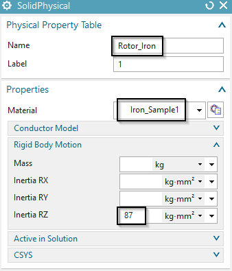
For the Rotor also create a tri mesh with the suggested size and
assign the material ’Iron_Sample1’. Also set the ’Inertia RZ’ to ’87
\(Kg mm^{2}\)’. Assign the name
’Rotor_Iron’.
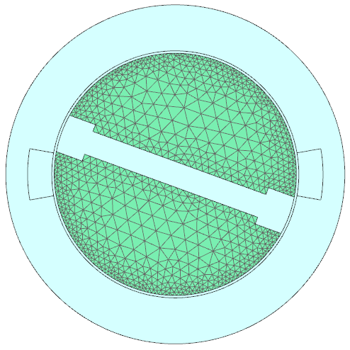
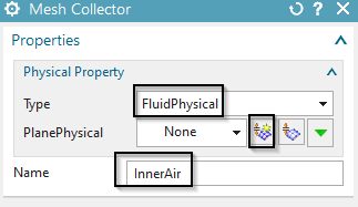
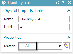
For the inner air (2 faces) create a tri mesh with suggested
element size and assign a ’FluidPhysical’ with material ’Air’. Name it
’innerAir’.
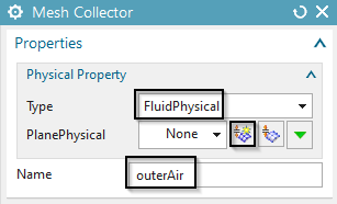
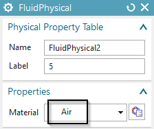
For the outer air create a tri mesh and assign one more
’FluidPhysical’ with material ’Air’. Name it ’outerAir’.
Notice: Do NOT mesh the air gap between rotor and stator. When
using the MovingBand feature this will be done automatically inside the
solver.
Check that all mesh collectors have a meaningful name. Then,
click the button ’Rename Meshes and Physicals from Collectors’ from the
Magnetics toolbar.
Switch to the Sim File.
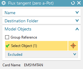
Assign a constraint of type ’Flux tangent (zero a-Pot)’ on the
circular edge of the infinity air.
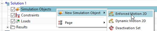
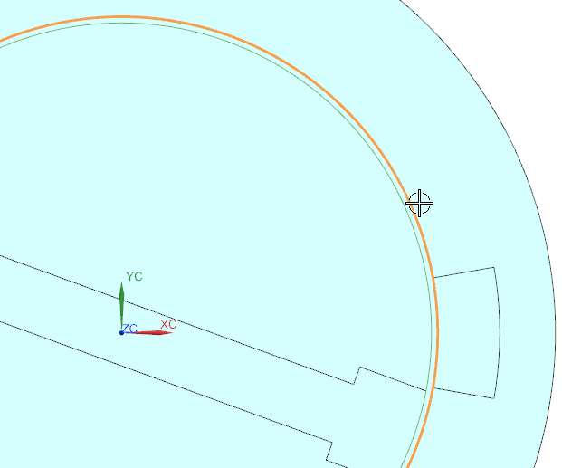
Now create a new Simulation Object ’Enforced Motion 2D’. Use the
type ’Revolute by Moving Band’. Hint: The type ’Revolute by General
Motion’ would also work, but this would use a different motion
technique.
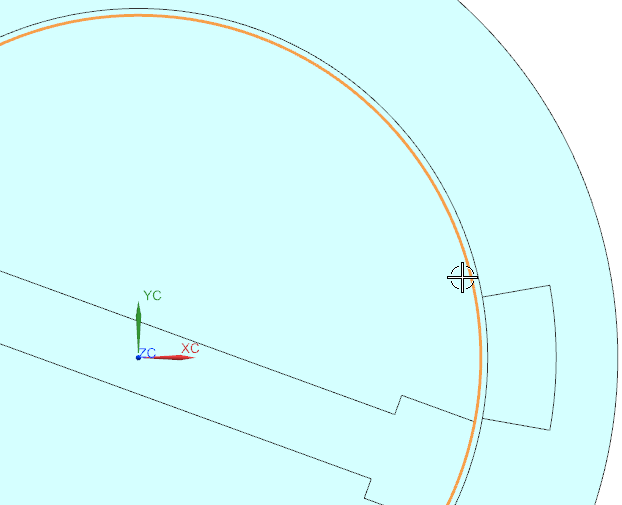
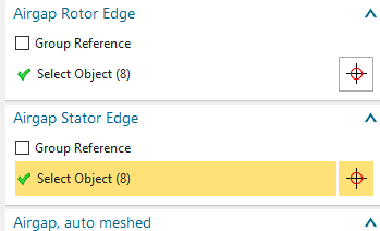
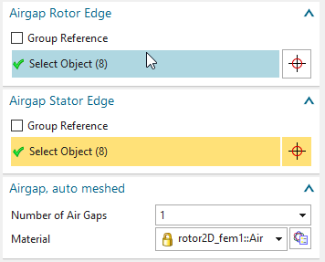
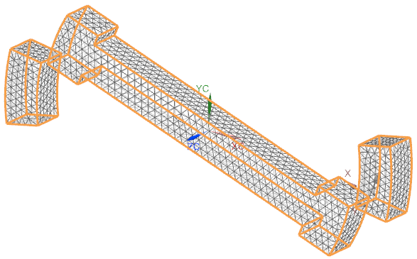
At ’Airgap Rotor Edge’ select the 8 inner circle edges as shown
below. These must be those edges, that belong to the moving part. Maybe
the selection filter with option ’Tangent Continuous Edges’ is helpful
here.
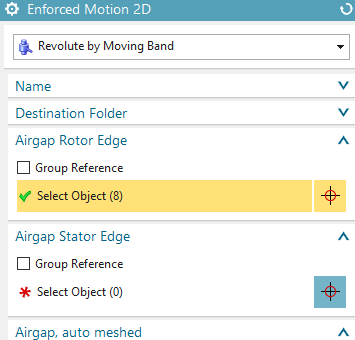
At ’Airgap Stator Edge’ select the 8 outer circle edges as shown
below.
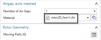
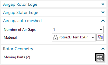
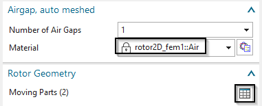
Under the box ’Airgap, auto meshed’ select from the list the Air,
that already resides in the Fem file. Accept the default 1 at ’Number of
Air Gaps’.
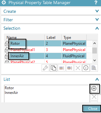
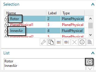
Under ’Rotor Geometry’, click ’Create Moving Parts’ and select the Rotor and the inner air and add these to
the list. Then click ’Close’ as shown below. If the names do not appear
in the list take care that in the Fem file the Physicals have such names
assigned.
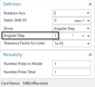
At ’Angular Step’ key in 1 deg. Because we have defined 45 time
steps we will compute for 45 degrees of motion with these settings.
OK.
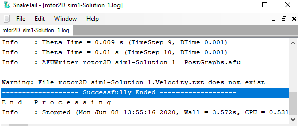
Solve the solution. The solution monitor indicates the progress
and successful end.
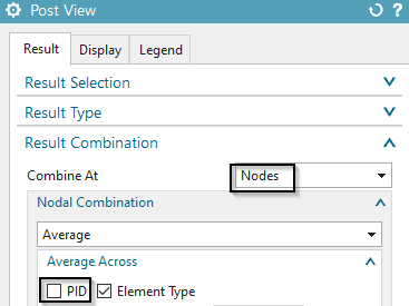
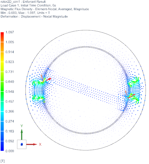
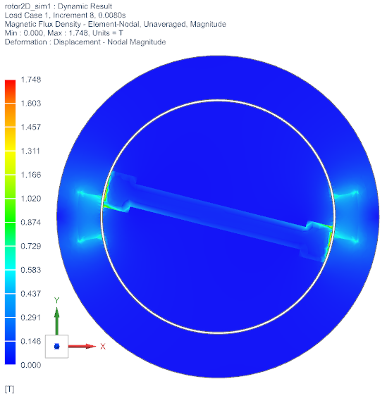
Plot the Magnetic Flux Density and observe the result. For a
smoother display set the ’Combine At’ option at ’Edit Post View’
to ’Nodes’ and at ’Average Across’ deactivate ’PID’.
The plot with magnetic flux density, arrows and contour, then
will look like the following for increment 1.
Cycle through the time steps by using the green button ’Next
Iteration’ . Alternatively, use the ’Animation’
function and set the option ’Animate’ to ’Iterations’. If you want to
see more movement repeat the solution with more time steps.
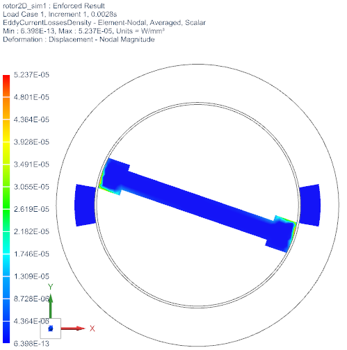
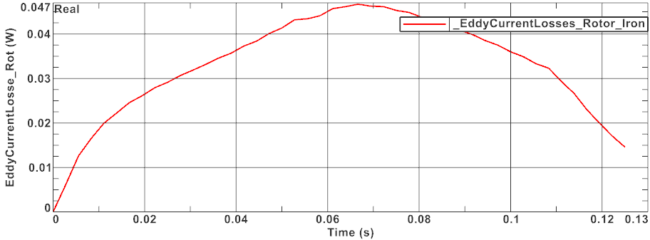
Display the eddy current losses on the rotor. This graph shows
nicely the eddy current effect when rotor and magnets move near to each
other.
This ends the tutorial.
2D Dynamic Driver
The following example is a pure 2D example; and particularly is
intended to be a follow-up example of the previous example ’Simple
Rotor, Enforced’. In this example, the rotor oscillates between two
permanent magnets. The example shows how to perform an analysis that
couples electromagnetics and mechanical movement. In the present
scenario the magnet is simulated with a dynamic motion. Here, the
movement has one degree of freedom in the mechanical sense. The example
is executed in 2D because of the shorter solution time but it would be
quite similar in 3D.
Main goal is to find the oscillation behavior of the rotator. Other
results like eddy currents can be requested additionally if
desired.
Estimated time: 25 min
Follow the steps to reproduce it:
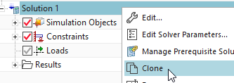
Start from the previous example and clone the solution,
then remove the enforced joint.
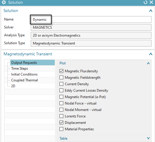
Name the new Solution ’Dynamic’.
Chose Analysis Type ’Magnetodynamic Transient’.
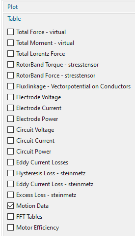
In register ’Output Requests’, Table activate ’Motion Data’ and
in Plot activate Displacement as well as ’Magnetic Fluxdensity’. Others
can be activated if desired.
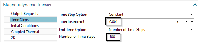
Modify the ’Time Increment’ to 0.001 and the ’Number of Time
Steps’ to 100 resulting in a total simulation time of 0.1 sec.
Change to the Sim file, if not already there.
If a new solution is created, add the constrain ’Flux Tangent’ to
the solution.
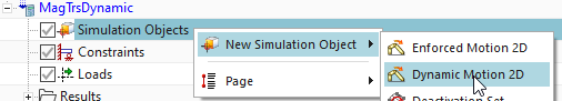
Create a ’New Simulation Object’ of type ’Dynamic Motion 2D’.
Remove the old one, if the solution was cloned.
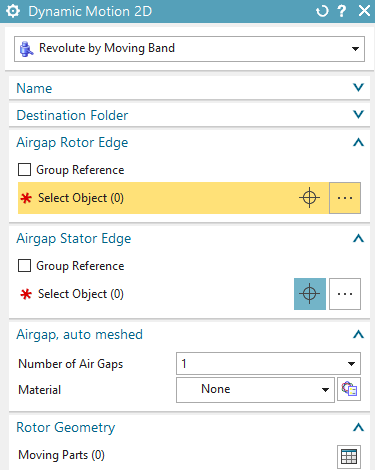
Select Type ’Revolute by Moving Band’ (the default)
Select the ’Airgap Rotor Edge’ and the ’Airgap Stator Edge’ in
the same way as already done in the previous enforced example.
Again select Air for the material at the Airgap
At ’Rotor Geometry’: Select the Rotor and the inner air.
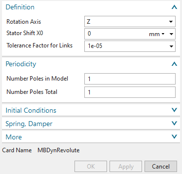
All other settings can stay at the defaults. There is no step
size necessary because this will be computed from the dynamics of the
system: Electromagnetic forces and mass inertia of rotor.
Solve the Solution. This will take about 1 min.
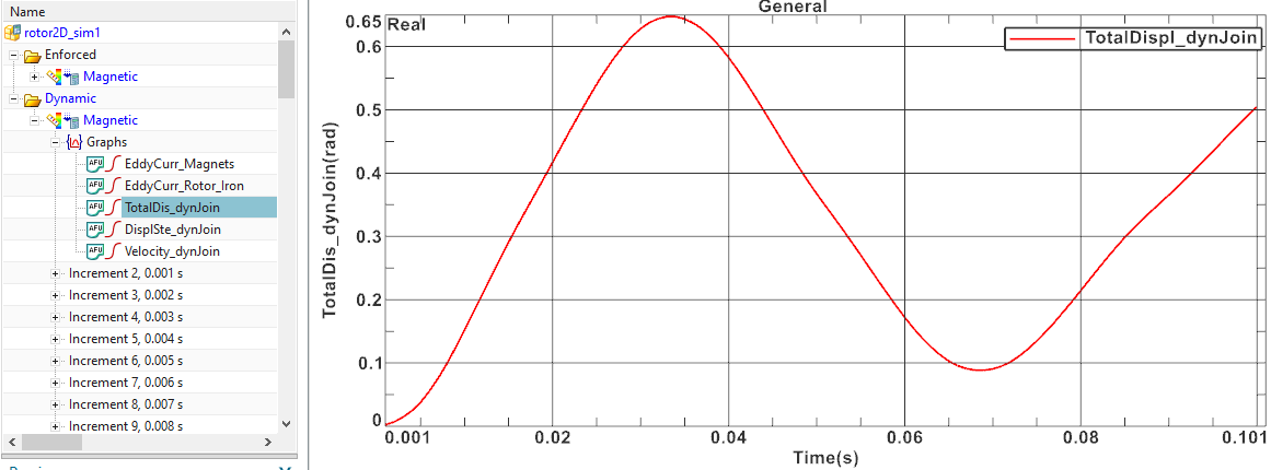
Now verify the oscillating behaviour of the rotor. To do so, open
the results and display the ’Total Displacement’ of the dynamic joint as
in the below picture.
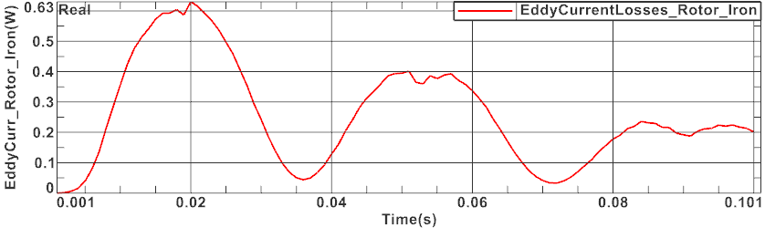
Also plot the graph showing the eddy current losses on the
rotor.
Then plot the Magnetic Flux Density.
This ends the tutorial.
3D Enforced Driver
In this example we will use an enforced driver and 3D geometry.
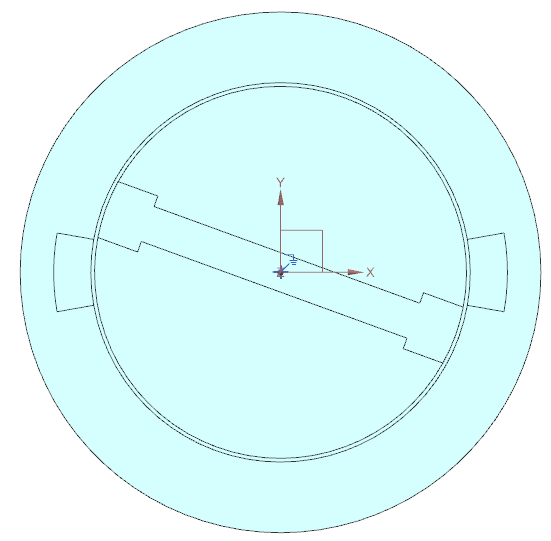
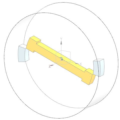
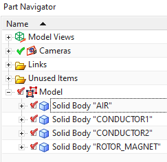
Estimated time: 1 h. The following picture shows the geometry and the
named CAD bodies.
Create a new FEM and Simulation. Choose Solver ’MAGNETICS’ and
Analysis Type ’3D Electromagnetics’. Switch off the ’Create idealized
Part’.
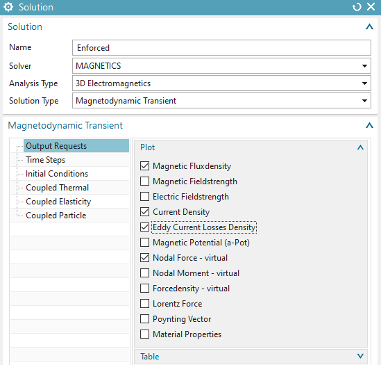
Choose Solution Type ’Magnetodynamic Transient’. Name the
solution ’Enforced’.
In register ’Output Requests’ under ’Plot’ activate ’Current
Density’ and ’Eddy Current Losses Density’ to enable the calculation of
eddy currents. Also enable ’Nodal Force - virtual’ to check for these
results.
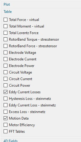
Under ’Table’ activate ’Eddy Current Losses’ to enable the
calculation of integrated current losses and to get them written into a
tabular file. Also enable ’Motion Data’ to get results of displacement
and velocity of the motion driver.
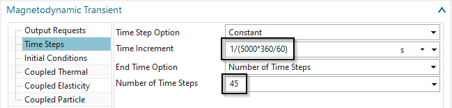
In register ’Time Steps’ set the ’Time Increment’ as shown. This
corresponds to a rotor velocity of 5.000 U/min if the step size is 1
deg. We will use this later.
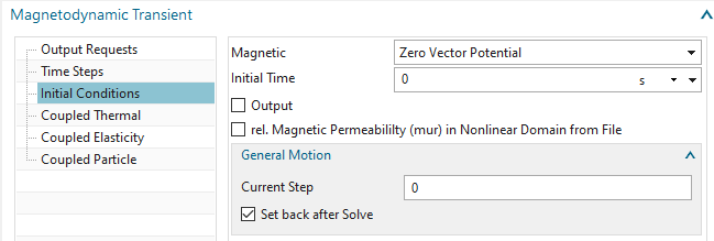
In register ’Initial Conditions’ accept the defaults. Hint: The
option ’Set back after Solve’ can be deactivated to allow restarting
from a previous run.
Click Ok.
Switch to the Fem file.
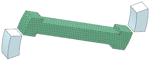
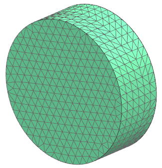
Mesh the rotor:
Use (3D) tetrahedral elements and the half of the suggested
element size.
Assign material ’Iron_Sample1’ from the Magnetics material
library.
Key in the value 87 Kg \(mm^{2}\) for Inertia RZ. This is necessary
only in case of dynamic motion of the rotor because the forces acting on
the rotor will be transformed into a motion step by Newtons
law.
name the collector ’Rotor_Iron’, click OK to finish.
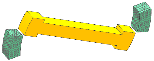
Mesh the two magnets:
Use (3D) tetrahedral elements with half of the suggested element
size.
Assign material ’N30EH at 100C’. Name the collector ’Magnets’.
OK. Hint: For the north direction, we want x. Because x is the default,
there is nothing to do now.
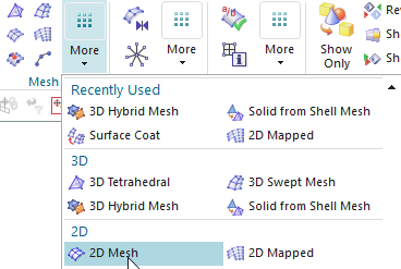
Mesh (2D) the three outside faces of the body ’AIR’.
Use (2D) tri elements with a quarter of the suggested element
size.
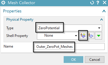
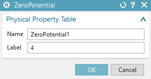
In the mesh collector of this 2D mesh, set the Type to
’ZeroPotential’ and click ’Create Physical...’. and OK. This setting
will impose a boundary condition at the mesh level, so there is no need
to give a zero potential condition in the Sim file.
name the mesh collector ’Outer_ZeroPot_Meshes’. OK.
Notice: This 2D mesh will be used two times: First it serves as boundary
condition and second it is used as border for the following air mesh
(Solid-from-Shell Mesh).
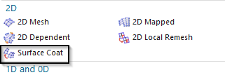
Now create 2D Surface Coat meshes on the parts:
Blank the 2D meshes and also the air body.
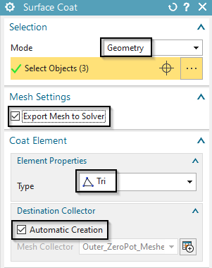
Choose the meshing function ’Surface Coat’,
Select the bodies of the two conductors and the rotor,
Set the ’Mode’ to ’Geometry’, activate ’Export Mesh to Solver’
and ’Automatic Creation’, Check that the ’Type’ is set to ’Tri’.
The system creates by default a physical of type NotToSolver what
is correct because we want to use these 2D meshes only as borders for
the following air mesh (Solid-from-Shell Mesh).
Assign the name ’Inner_Coat_Meshes’ to this mesh collector.
We want to have all collector names written to the corresponding
physicals and meshes because this is easier to use. Therefore click the
button ’Rename Meshes and Physicals from Collectors’ from the Magnetics
toolbar.
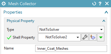
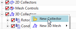
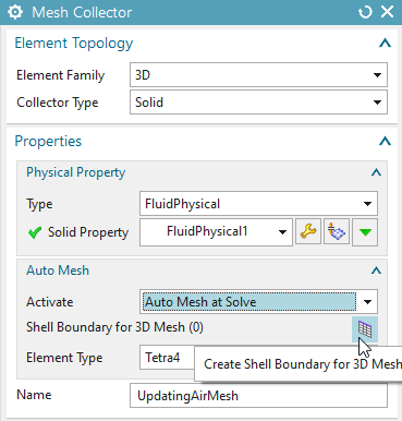
Next we create a new 3D mesh collector that will later hold the
3D air mesh. We will set up this collector in a way that it
automatically updates the air mesh at every new rotor position. It will
automatically use the ’Solid from Shell’ mesher, therefore it is
necessary to have meshed the 2D border of this 3D air.
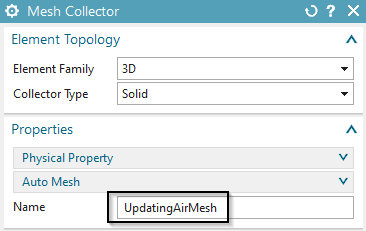
First choose the function to create a new collector.
Name this collector ’UpdatingAirMesh’.
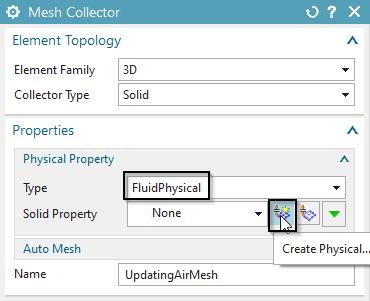
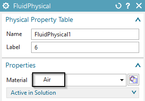
In box ’Physical Property’ set the ’Type’ to ’FluidPhysical’. Use
the button ’Create Physical’ to create a new physical. In the new
physical choose the material Air. OK.
Back in the mesh collector dialogue expand the box ’Auto Mesh’
and set the option ’Activate’ to ’Auto Mesh at Solve’.
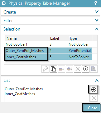
Next choose the button ’Shell Boundary for 3D Mesh’. In the
following dialogue select the two border physicals and click on
’Add’.
Then press Close and Ok to close all dialogues.
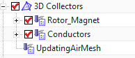
The navigator now shows the new collector. Notice that there is
no mesh in it. This mesh will be created at solve time automatically
through the function ’Solid from Shell Mesh’. The mesh will also be
updated at every motion step.
Switch to the Sim-file.
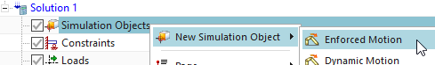
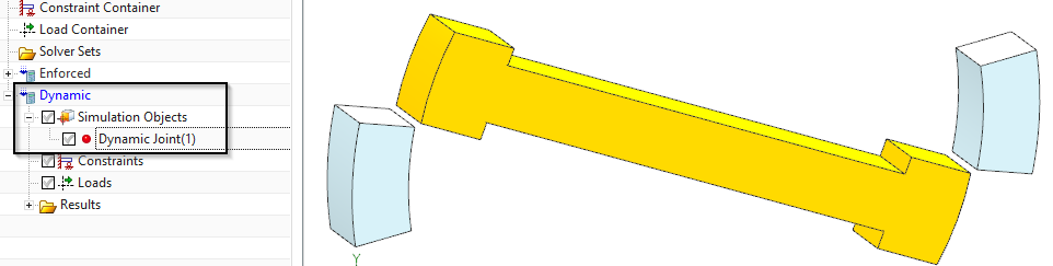
Create ’Simulation Object’ for the rotor movement:
Choose the function ’Enforced Motion’. The following dialogue
appears
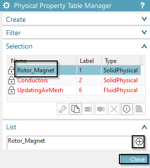
At ’Rotor Geometry’ click on ’Create Moving Parts’ . In the following dialogue select the physical
Rotor_Magnet and click Add, Close.
Notice that the ’Angular Step’ is set to one degree for each
step. This is already what we want so there is no change necessary.
Leave all other settings at their defaults. OK.
Hints: By this procedure the MAGNETICS Solver will rotate the 3D
Rotor mesh at each timestep for the desired amount and will
automatically create ’Solid from Shell’ meshes for the air using the
previously created 2D boundary meshes.
Model setup is now done. Save your parts, blank the meshes (maybe
you leave the rotor mesh visible because this will nicely show the
motion). Decrease the window size, because it will pop up to foreground
at every time step.
Solve the solution. This will take 5-10 minutes because of the 45
steps to run. A progress bar at the bottom of the Simcenter window shows
the current and the remaining steps.
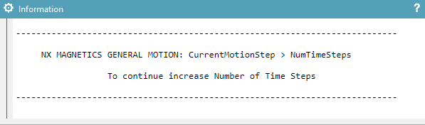
The finishing of the solve is shown by the information window as
below
After the solve finishes you can post process the results.
Open the plot results. All motion steps are stored in the result
file. This allows running animations over the iterations and creating
movies if desired.
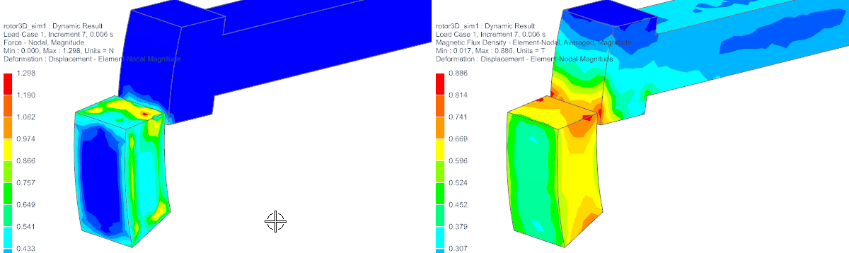
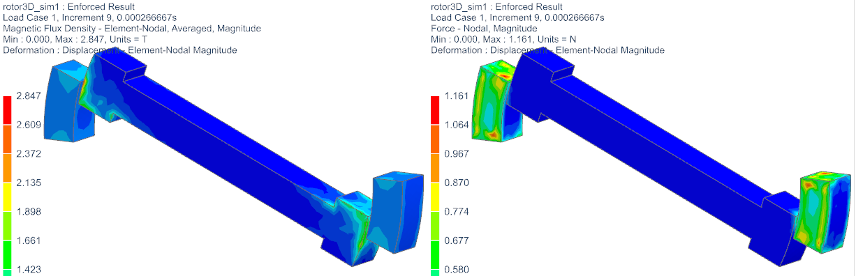
The following picture shows the magnetic flux density result
(left) and the nodal forces (right) at time step 9. (Results are set to
averaged at nodes and element edges are blanked).
After this General Motion run the moving meshes are set to
’Locked’. If an update of the meshes to the original situation is
desired, unlock the moving meshes and perform a mesh update.
The tutorial is complete.
3D Dynamic Driver
The completed Sim file, that resides in the tutorial folder, contains
also a solution (named ’Dynamic’) with a dynamic joint. This can be used
for further studies. (Set the ’Number of Time Steps’ to 100 before
solving the complete period.) The following result graphs are made with
a larger number of time steps. Of course, that solution needed much more
time.
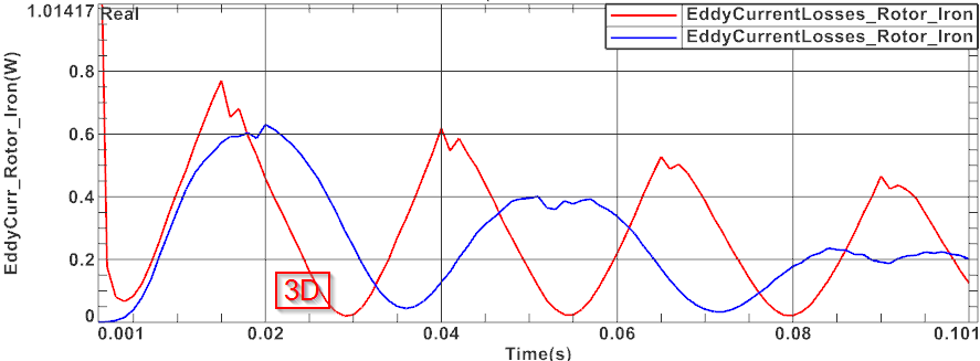
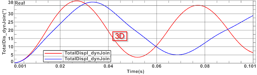
The following picture shows the resulting displacement of the previous
2D dynamic (blue) and the 3D dynamic (red) rotor. The next picture shows the resulting
eddy current losses of the 2D dynamic (blue) and the 3D dynamic (red)
rotor.
When comparing the 2D and 3D results one will find out that the
simulated forces and torques are higher in the 3D case, even if the 2D
is set to the same z thickness. Therefore, also the dynamic rotation
speed becomes higher in 3D. This effect can be explained as follows: The
magnetic forces appear mainly on the border faces between air and
magnetic material. Because the 3D model has additional side faces, and
these are used in the simulation, the forces here are higher. The
following picture illustrates this: It shows the force distribution on
the 3D rotor. It can be seen, that forces are not homogeneously
distributed. At the side faces they are higher. Also the magnetic flux
density result shows this effect. This is one reason why 3D simulations
can be more realistic.


 The next picture shows the resulting
eddy current losses of the 2D dynamic (blue) and the 3D dynamic (red)
rotor.
The next picture shows the resulting
eddy current losses of the 2D dynamic (blue) and the 3D dynamic (red)
rotor.