This tutorial shows a basic simulation principle of electric switches. Two conductors initially are in contact and electric current is flowing through both. Then, a mechanical force is acting on one of them forcing the contact to open and the current to stop. Even in the closed situation, there is a very small air gap in the contact area and this does produce some electric resistance. While the contact gradually opens, this gap enlarges and the resistance quickly becomes very high, so the electric current stops crossing the contact.
Estimated time: 0.5 h.
Follow the steps:
First check the existing model files of this tutorial.
Download the model files for this tutorial from the following
link:
https://www.magnetics.de/downloads/Tutorials/8.CouplStructural/8.4TouchingConductors.zip
Open the file ’TouchingConductors_sim1.sim’-
Delete the Simulation Object ’Thin Gap Condition(1)’ and also the Modeling Object ’Elasticity Contact Parameters1’. We will newly create these in the following.
Check the existing model: First set the Fem part displayed to see the content.
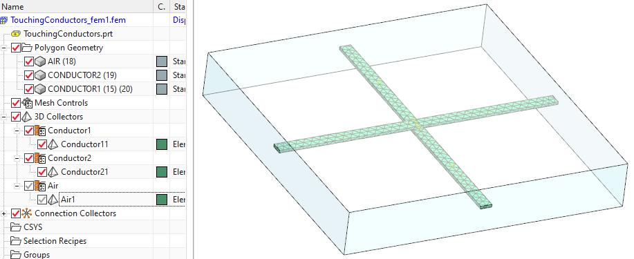
There are two conductor meshes and one air. Nothing is special. It is very similar to the previous tutorials with electric conductors.
One thing should be noticed: The Mesh Mating Condition between the two conductors is also a usual condition of type ’Glue Coincident’. Until now the two conductors are treated as if they were one. Later in the Sim file, we will define a ’Thin Gap Condition’ with coupling to elasticity here. Thus, this face will become a contact that allows to open.
Set the Sim part displayed and check the solution.
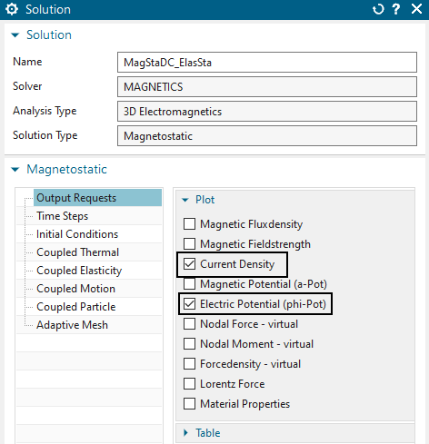
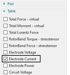
Edit the existing solution ’MagStaDC_ElasSta’ to check the settings. It is a magnetostatic solution type with some basic output requests activated to check the current.
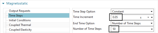
in ’Time Steps’ there are 50 steps with 0.05 sec defined. During this time period the mechanical force will act, first forcing the closing direction, then altering to the open one.
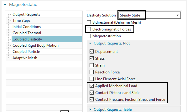
In ’Coupled Elasticity’ the ’Elasticity Solution’ is set to ’Steady State’ and some output request for contact are activated. Although this is a static solution, all these features are also possible in transient solutions.
Notice, ’Electromagnetic Forces’ is deactivated. Of course, this can also be active. But in this tutorial we want to see the effect of mechanical forces only.
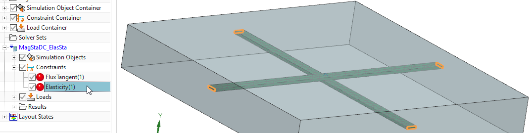
Check the constraints.
Like always in electromagnetics, there is a ’Flux Tangent’ condition at the outside walls of the meshed volumes.
An elasticity constraint ’Elasticity(1)’ fixes all four electrode faces of the two conductors.
Check the loads.
There is a current load ’Current(1) Static’ applied to one of the electrode faces. This injects an electric current of 50000 amps into the conductor system. All three remaining electrode faces have a voltage zero condition applied that allows the current to enter or leave.
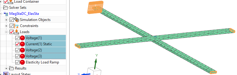
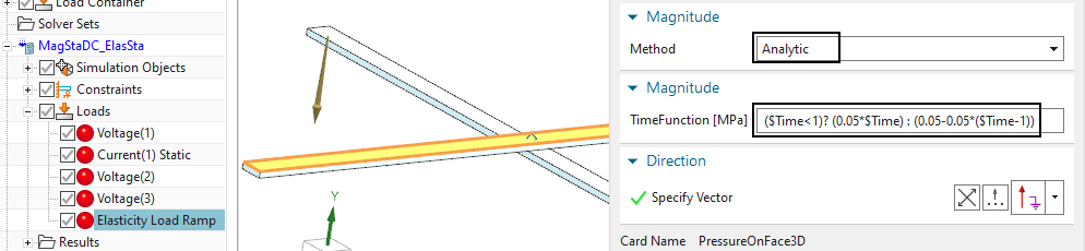
A mechanical pressure load named ’Elasticity Load Ramp’ is of
’Analytic’ type and uses the following time dependent condition:
\((\$Time<1)? (0.05*\$Time) :
(0.05-0.05*(\$Time-1))\).
This form reads as: In case time is smaller 1, use the form \(0.05*Time\). In other cases, use the form
\(0.05-0.05*(Time-1)\). These are two
linear functions, one for the increase the other for the decrease of the
mechanical pressure.
Such were the existing features in the model. Nothing very new for the readers of this document. Following the new condition is created.
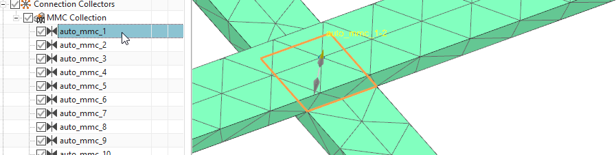
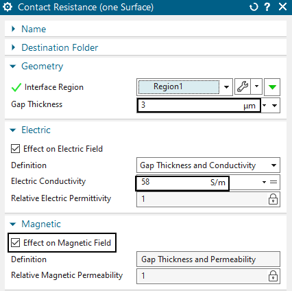
Create a new Simulation Object ’Contact Resistance (one Surface)’.
At ’Region’, select the contact face between the two conductors.
Set the ’Gap Thickness’ to 0.003 mm. This value represents the initial gap opening. There is already a small electric resistance because of this small gap.
Activate ’Effect on Electric Field’ and set the ’Electric Conductivity’ to the value 58 S/m. Notice, this is much less than copper with 58e6 S/m. Thus, as long as the gap remains small there is very small resistance.
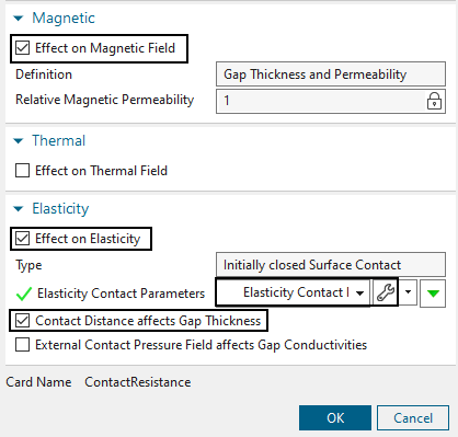
Also activate ’Effect on Magnetic Field’.
Now activate ’Effect on Elasticity’ and create a ’Modeling Object’ for contact parameters (accept all defaults here).
Finally, activate ’Contact Distance affects Gap Thickness’. This leads to the desired effect of stopping the current when opening the contact.
Solve the solution. The 50 steps with contact need about 2 minutes solve time.
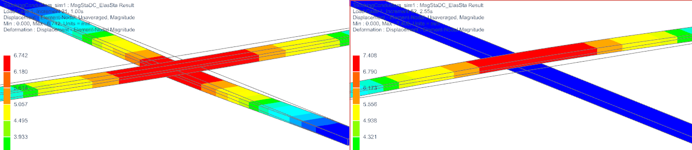
Display the Displacement results. Tip: For easier display, hide the Air mesh and also set the edges to ’Feature’. In the below picture there are additionally the undeformed edges shown. The left side shows the time of full force in contact direction. The right side shows the time of full force in opposite. The gap arise can be clearly seen.
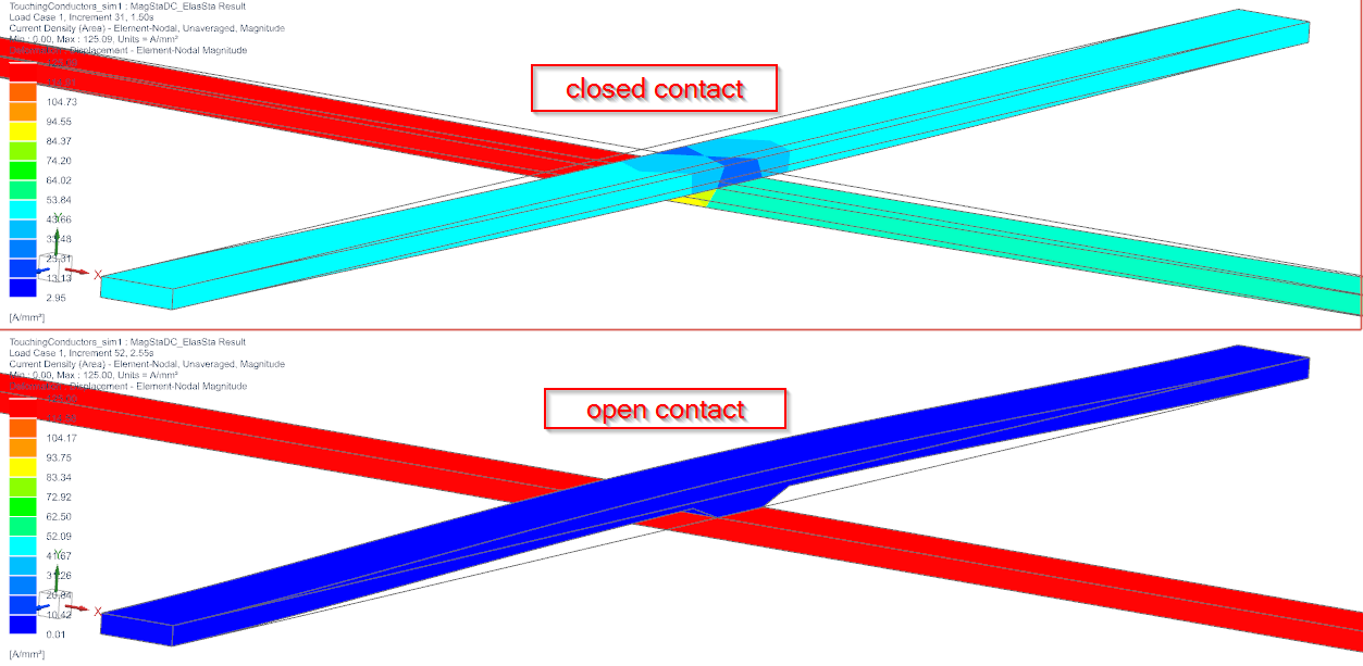
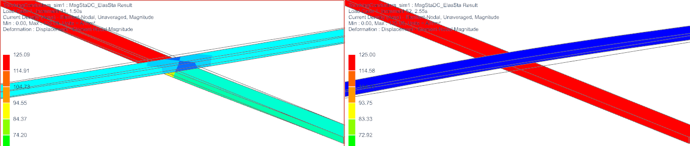
Set the result to ’Current Density’ now. Again, compare the two time steps as in picture below. Left side is the closed situation and the electric current being injected (top left) is split in three parts. Right side shows the open situation. The whole current now flows through one conductor.
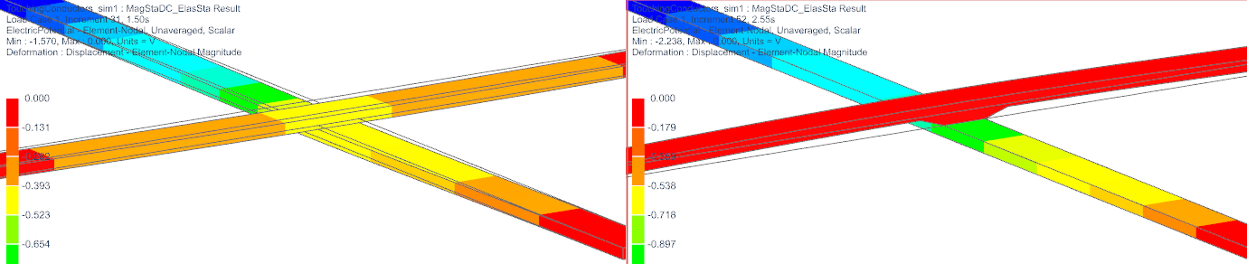
Finally, set the result to ’Potential’ and again compare. Left side (closed) shows there is no jump in the potential at the contact. Right side (open) does show the potential jump.
The tutorial is finished.