This tutorial shows a simple electro mechanical switch and its
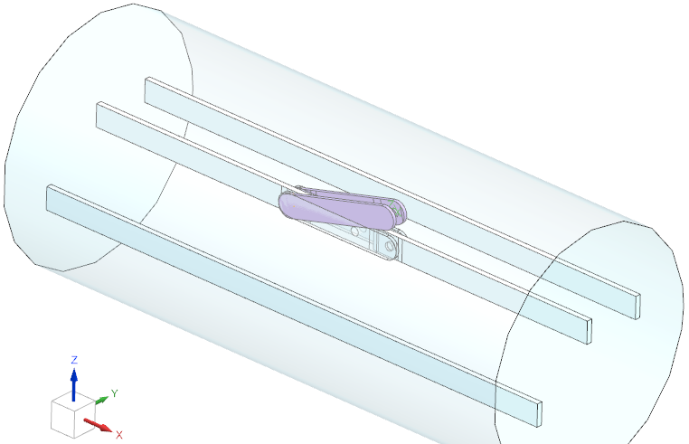
simulation principle. Three conductors are arranged as shown below
(left) and loaded by three phase AC currents. For simplicity in this
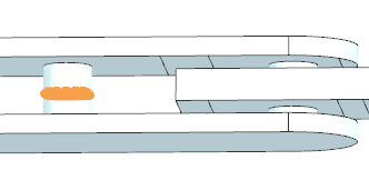
tutorial, only one of the three has a switch. The switch is shown in
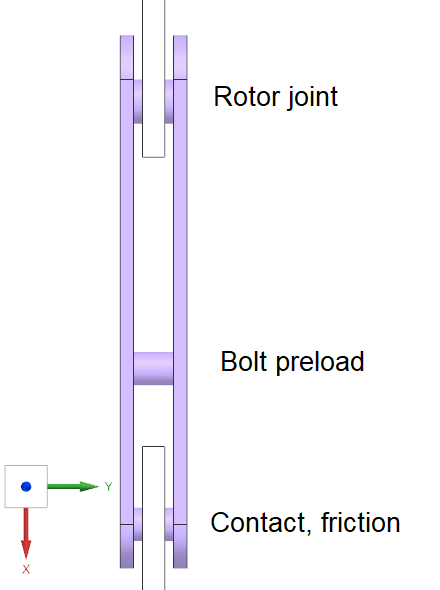
detail below right. A free rotating joint connection without friction
couples the switch to the conductor (top). On the other side (bottom) a
clamped contact with friction connects to the other conductor side. In
between there is a cylinder with mechanical pre-load, for instance by a
screw. The pre-load is given, also the friction coefficient and the
electric currents.
Lorentz forces acting on the conductor system will maybe open up the
switch and therefore this simulation shall give an estimation about
expected movements of the switch.
Estimated time: 1 h.
Features to learn:
Elasticity Contact with effect on electric and magnetic field,
Elasticity joint connections,
Elasticity Bolt pre-load.
First check the existing model files of this tutorial. This model is completely set up with all necessary features. In the tutorial we walk through those features of interest and discuss them. Of course, a good idea for learning would be to start from the CAD model (in folder ’start’) and set up the whole model.
Download the model files for this tutorial from the following
link:
https://www.magnetics.de/downloads/Tutorials/8.CouplStructural/8.5SimpleSwitch.zip
Open the file ’SimpleSwitch2_sim1.sim’.
Check the existing model: First set the Fem part displayed to see the content.
The first thing to draw the attention on is the rotating joint
connection and how this is managed in the model. Often in
electro-mechanical devices there are components being coupled in that
way: only rotation is possible what is also called a revolute joint. One
possibility for such a connection can be using several contacts. But
another, simpler possibility is the construction of several line
elements like we do here. Line elements in elasticity behave like rods,
that means they do not transfer moments.
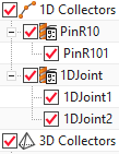
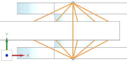
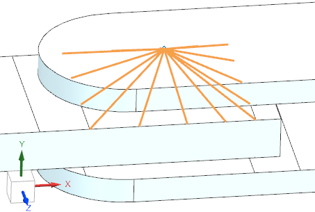
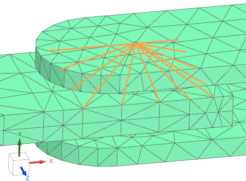
The pictures below show that type of joint model that is a build by two
’Spider’ type 1D connection meshes, each from a point to some edges.
Additionally there is one direct 1D connection from point one to point
two. By using such a construction the parts are connected by the lines,
but rotation is allowed.
The material ’JointMat’ and physical properties for such joint elements are chosen in a way that they do not influence the dynamics: they have a very small mass and the elastic modulus is taken from steel. The ’Tube Radius’ is chosen in a way that the elastic forces will be strong enough to keep the parts in position. We would notice by the resulting displacements if these are chosen too small.
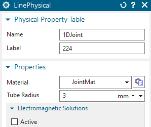
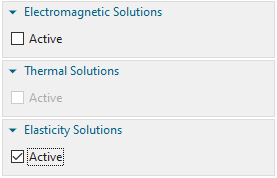
For the lines all solutions but ’Elasticity’ are deactivated, so they do not play a role for the electromagnetic solution.
Lets now check and discuss the bolt pre-load, so set the Sim part displayed.
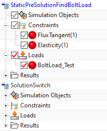
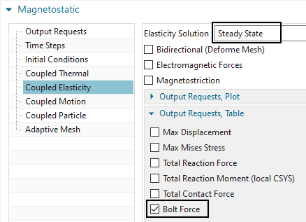
Notice, there is a solution named ’StaticPreSolutionFindBoltLoad’. This is a simple Magnetostatic solution with all constraints, but no contacts. Coupled Elasticity is set to ’Steady State’ here.
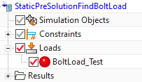
There is also a load ’BoltLoad_Test’. This is an ’EM Elasticity Load’ of type ’Bolt Pre-Load on 3D Elements - Cut Plane’.
As the names announce, we use a pre solution. The bolt load feature
currently cannot directly use a force as input, instead it can use a
given displacement (similar to negative strain) on the bolt. That
enforced displacement or strain will result in force. Thus, the strategy
is applying an initial displacement, finding the resulting force and
scaling the displacement to the desired bolt force. The corresponding
displacement leading to that force will be the needed one for following
simulations.
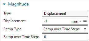
In this tutorial the desired bolt load is 5000 N. In the pre-solution we
initially apply a displacement of -1 mm. Notice, the ’Ramp over Time
Steps’ is zero. This option is useful only in dynamic solutions, to
prevent unwanted oscillations.
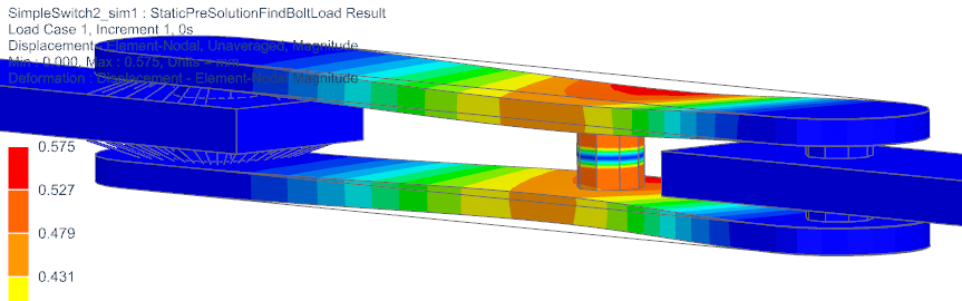
Thus, after solving, there results a deformed bolt and the tabular result shows the bolt force is 8191.6 N (the plot below shows an over scaled deformation).
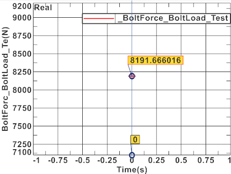
To find the necessary scaled displacement we divide the desired 5000 by 8191.6 what results in a scale of 0.6104. Thus, in the main solution ’SolutionSwitch’ we use -0.6104 mm as applied displacement. Also, in that dynamic solution, we use a ’Ramp over Time Steps’ set to 5 to avoid oscillations.
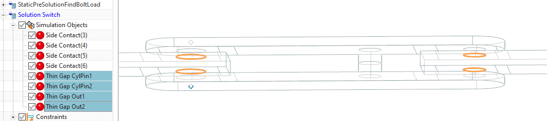
Notice the Simulation Objects named ’Thin Gap CylPin’ and ’Thin Gap Out’. These define faces at which electric current passes over a gap and that gap may change its thickness and size depending on the elasticity solution. These contacts work as already demonstrated in the previous tutorial ’8.4TouchingConductors’.
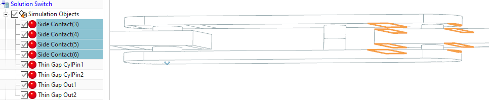
Beside the contacts with EM Elasticity Coupling there are also some other contacts that simply avoid penetration of the geometry while deforming. These are the Simulation Objects named ’Side Contact’. They are of type ’Elasticity Contact’ and they work as already demonstrated in the previous tutorial ’8.3ElasticityContact’.
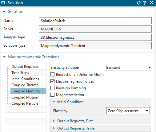
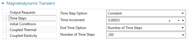
Finally, check solution ’SolutionSwitch’. There is nothing special in it. It is a Magnetodynamic transient one with Elasticity coupling also set to transient.
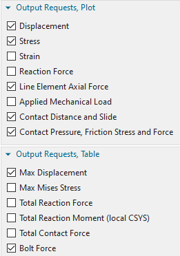
Time Steps and time increment are shown below. Set the ’Number of Time Steps’ to 200 to solve the full range. Some usual output requests (Plot: Current Density and Table: Electrode Current) are activated.
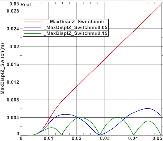
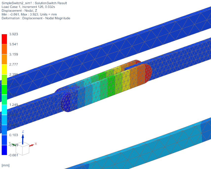
The solve of these 200 time steps with EM Elasticity coupling will take about 30 minutes. Main results of interest are displacement over time steps. Also the moment that results from lorentz forces and acts on the switch is of interest. The following graphs show the Z displacement of the switch (red curve) and the moment around the axis (blue curve). The left picture shows the maximum displacement of the switch.
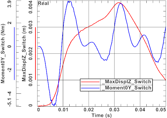
The above simulation shows relatively small displacements of the
switch. That can be explained by the behaviour of the moment what
results from the given oscillating voltage load.
The tutorial is complete.