This tutorial shows how electric conductors contact while deforming. A later tutorial additionally shows how contacts can influence the electric current, what means if a gap arises, the electric resistance becomes very large. This example only shows the mechanical effects.
Follow the steps to see how the model is set up, solved and how the
contact can be managed. The tutorial starts from an existing Fem and Sim
file. Only the relevant features are added.
Estimated time: 1 h.
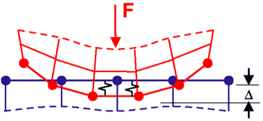
We use a classical elasticity contact feature, also called penalty contact algorithm. That feature introduces nonlinear mechanical effects what means that at each time step the solver must check for penetration in the contact area and if such penetration appears, there will be contact forces added. The contact forces must be adjusted in a way that the penetration disappears or falls below a given limit. To find such correct contact forces the solver must perform several iterations. Because of these extra contact iterations the computational costs become significantly larger when using contact.
Two contact types are possible: ’Node-to-Node Contact’ and ’Surface-to-Surface Contact’. The first type can be used to define single contacts between two points in the model. The second type is more advanced and can also handle coulomb friction. In this example we use both types for completeness.
First check the existing files of the tutorial.
Download the model files for this tutorial from the following
link:
https://www.magnetics.de/downloads/Tutorials/8.CouplStructural/8.3ElasticityContact.zip
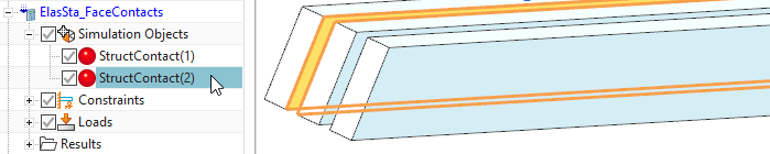
Delete all existing ’Simulation Objects’. These contacts will be created in the following.
Check the existing model:
There are meshes of different types just to make sure contact work on all of them.
Two solutions are already there. One will be used for face
contact and one for node contact. The solutions are of Magnetostatic
type with zero time steps and we are only interested in the elasticity
part.
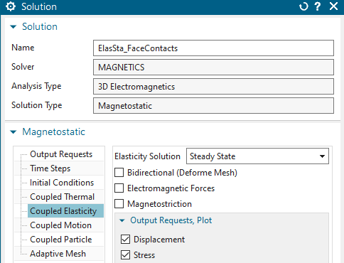
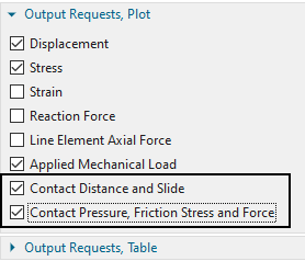
Notice there are two ’Output Requests’ activated for this contact simulation: ’Contact Distance and Slide’ and ’Contact Pressure, Friction Stress and Force’.
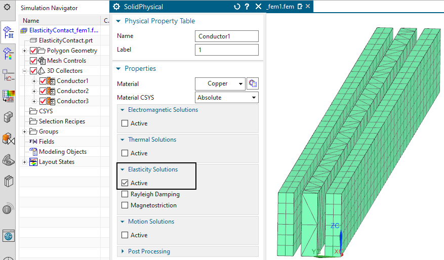
The Physicals of all conductors also show that only the
elasticity solution is of interest. All others are deactivated. The
material is copper with an standard elastic modulus and poisson
ratio.
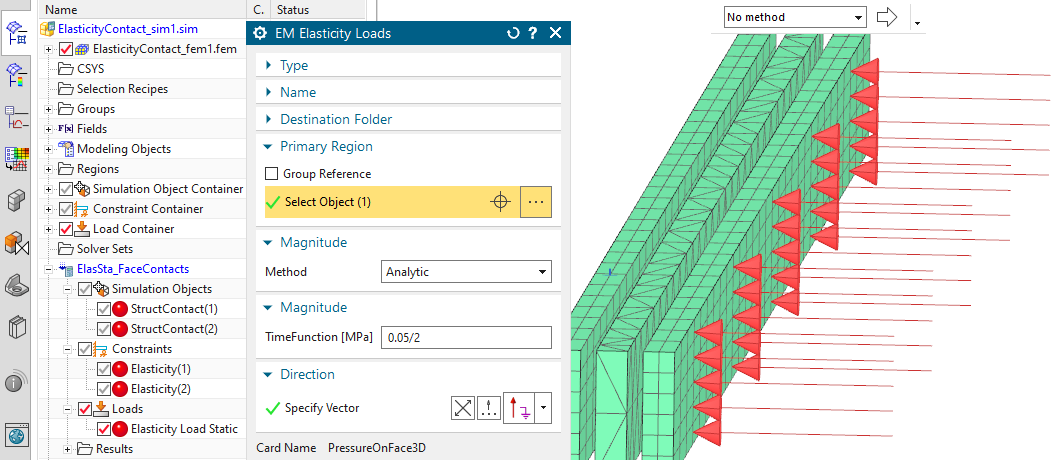
There is a pressure load working on one side of a the first
conductor. Without contacts, this load would lead to a large penetration
(Solve to check this). Also some elasticity constraints are defined to
hold the three conductors in place.
Create the first face contact as follows
In ’Simulation Object’, choose ’Elasticity Contact’ and set the
’Type’ to ’Surface-to-Surface Contact’. Now the two contact regions are
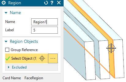
defined. At ’Source Region’, click ’Create Region’ and select the face
as shown below.
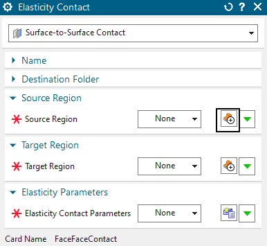
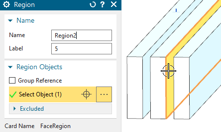
At ’Target Region’, again click ’Create Region’ and select the
opposing face.
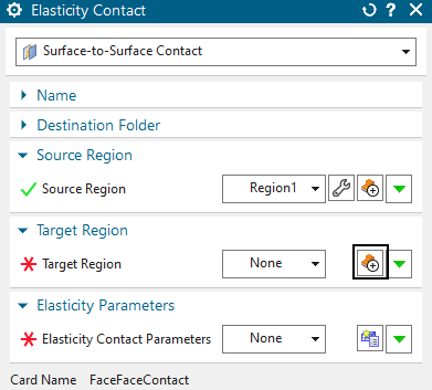
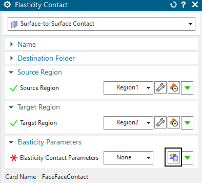
At ’Elasticity Contact Parameters’, click ’Create Modeling
Object’. The coefficient of friction, damping and several numerical
parameters can be modified here. In many cases the defaults work fine,
so there is no need to change anything now. Click OK two times to finish
the contact creation.
Create the second contact in the same way between conductor 2 and
3 and their corresponding faces.
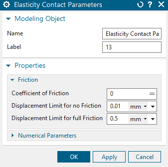
Even if we did not modify any, we will give a short information about the above contact parameters, because they definitely influence the simulation process. Although, many models run with the defaults, often solve time can be reduced by adjusting contact parameters.
’Coefficient of Friction’: This value controls the coulomb friction forces that appear if this value is set larger than zero. Such friction forces act on the two contact faces in opposing directions, depending on the relative motion (slide). To control friction, there are also the two limits ’Displacement Limit for no Friction’ and ’Displacement Limit for full Friction’. The assumption is that friction forces do not appear suddenly, rather than gradually increasing depending on the slide distance. Though, the first limit defines a small slide range that does not produce any friction forces. Then, if slide increases, the range between limit 1 and limit 2 defines the slide range in which the friction coefficient arises linearly between zero and the full given value. If slide becomes higher, full friction stays in effect.
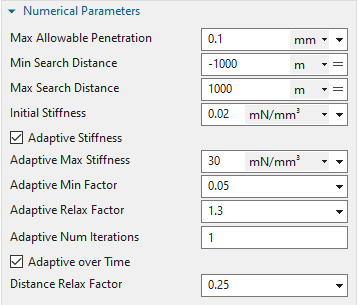
’Max Allowable Penetration’: This maximum penetration value defines the limit or residual that must be reached for a contact to converge.
’Min/Max Search Distance’: The algorithm searches from the source to the target faces (and opposite) to find contact penetrations. These two distances define the limits of that search. They shouldn’t be too small because often there is large penetration at the beginning of a contact process and even then the limits must fit.
’Initial Stiffness’ and ’Adaptive Stiffness’: The contact algorithm finds penetration and calculates contact forces by the amount of penetration times a stiffness factor. If ’Adaptive Stiffness’ is not activated, the used stiffness stays always the initial value given here. If the adaptive feature is activated, the stiffness factor will update depending on the current contact force, penetration and on the ’Adaptive Relax Factor’.
’Adaptive Max Stiffness’: If the adaptive stiffness feature is used this value controls the maximum possible stiffness.
’Adaptive Min Factor’: In case gaps arise during the contact iterations, the contact pressure will not suddenly become zero, rather it will decrease depending on the ’Distance Relax Factor’. As soon as the ’Adaptive Min Factor’ is reached, the pressure is set to zero.
’Adaptive Relax Factor’: This relax factor can be used to influence the adaptive stiffness computation. A smaller value, e.g. 0.1 leads to smaller stiffness, a higher value, e.g. 5. leads to more aggressive stiffness increase.
’Adaptive Num Iterations’: This factor defines whether the adaptive stiffness is updated once at the beginning of a time step only (Default) or if it is updated again at following iterations.
’Adaptive over Time’: If active, the previously adaptive stiffness is used at the beginning of a new time step. If not, it is initialized with the initial stiffness value.
’Distance Relax Factor’: This factor controls how aggressive stiffness is decreased if gaps arise in contacts. Normally, the default should not be changed.
Some more settings for contact are found in the solver parameters under register ’Numeric’ in box ’Nonlinear Elasticity Contact’. These are global settings, being valid for all contacts. If the setting ’Method’ is switched from ’Program Controlled’ to ’User Set’ one can modify them. To see more info in the following simulation, we set the ’Logfile Output’ to ’All’. Following the meanings of the settings.
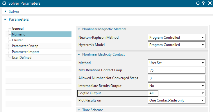
’Max Iterations Contact Loop’: Defines the maximum number of contact iterations. If the residuals of all contacts are not below their limits after these iterations, the whole step has not converged.
’Allowed Number Not Converged Steps’: Sometimes some contact residuals do not fully reach their limit but the overall solution is valid. Therefore, this parameter defines how many of such not converged (connected) time steps are allowed until the solution stops. The solution monitor indicates such steps with ’NOT converged - Continue’.
’Intermediate Results Output’: Setting this option to ’All’ leads to a result output at all contact iterations. This can be used for debugging purposes mainly.
’Logfile Output’: By default this is set to ’Mini’, meaning the solution monitor shows information about each final contact iteration. Setting this to ’All’ results in showing each iteration in the solution monitor.
’Plot Results on’. By using the default option ’One Contact-Side only’, contact results like pressure, force, sliding,... are shown on the first side of each contact only. Normally, the second side will have the opposing values and therefore it is not necessary to show such. Nevertheless, setting this option to ’Both Sides’ will show the results on both contact sides.
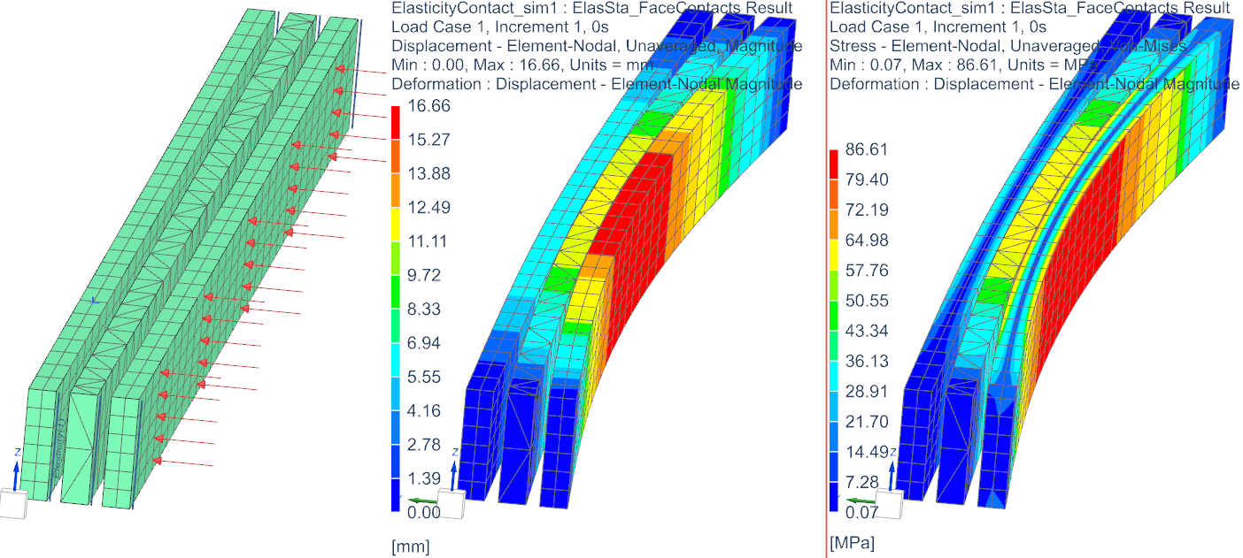
Solve this solution ’ElasSta_FaceContacts’.
The solution monitor gives information about contact iterations. Each line ’Contact Loop’ shows one iteration. The last line indicates that 62 iterations have been necessary for convergence.
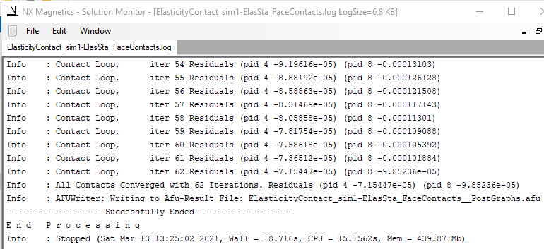
Also, each contact is shown in brackets with its property identifier ’pid’ and the residual. Negative values indicate penetration and positive values show distance gaps. Small penetrations below the limit have converged. The number of necessary iterations can be reduced by using larger contact stiffness, but in that case the risk for no convergence will arise.
Open the plot results and display the result ’Displacements’.
Verify that the overall solution looks correct.
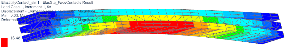
Also check the contact results. Display ’Contact Normal Force’, ’Contact Pressure’, ’Contact Slide’, ’Contact Distance’
In the second solution ’ElasSta_NodeContacts’ we want to use node contacts instead of face contacts.
Activate the second solution.
Create a new ’Simulation Object’ of ’Elasticity Contact’ and use the type ’Node-to-Node Contact’.
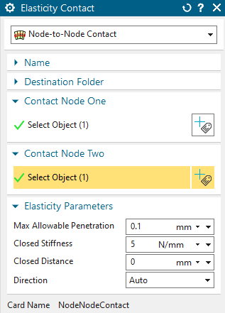
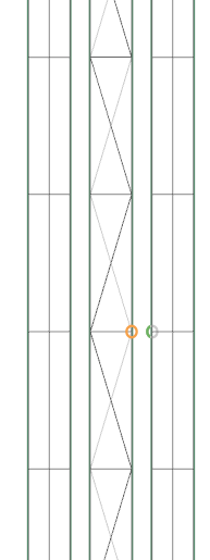
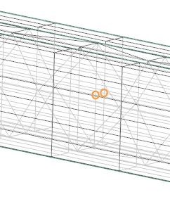
At ’Contact Node One’ select a node from the face of conductor one quite in the middle.
At ’Contact Node Two’ select a node from the face of conductor two quite in the middle. Click OK and the contact is created.
Create a second node contact between conductor two and three.
Solve the solution and post process the results.
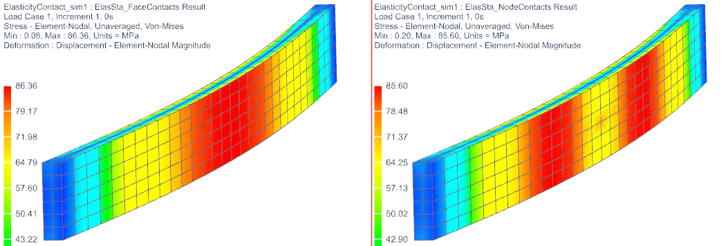
Deformation results will be similar to the face contact solution.
When comparing stress results, a difference is found. Because the node contact (picture below right) loads all contact forces on only the single node a different stress distribution results.
The tutorial is finished.