Dynamics of Three Conductors

The 3 phase conductor system we analyse in this tutorial is loaded by either DC, AC or by a formula based short circuit condition. We want to analyse for the electromagnetic fields and mechanical deformations, stresses and reaction forces that result from said three load types.

Due to Amperes law, each conductor will create a rotating magnetic field around himself, that also influences each other conductor. The smaller the distance between them, the higher is this effect. In case the conductors deform large, the distance between them will either increase or decrease and thus, the produced fields will also change. This nonlinear effect can be captured by bidirectional simulation: The EM fields modify the geometry, the changed geometry results in a change of the EM field.

So, we will first create the Fem model with meshes and material properties, nothing very special. Then we will create solutions for electromagnetics with static (DC load), frequency (AC load) and transient (short circuit load). For each solution we will add coupled elasticity and finally we will run a solution with bidirectional coupling and compare the results.

Estimated time: 1.5 h.

Follow the steps:

File Structure Setup

1. Download the model files for this tutorial from the following link:
   https://www.magnetics.de/downloads/Tutorials/8.CouplStructural/8.2ThreeConductors.zip

2. Open the file ’ThreeConductors.prt’.

3. Start Simcenter Pre/Post, Create a ’New Fem and Simulation’, use Solver MAGNETICS and Analysis Type ’3D Electromagnetics’. Switch off the ’Create Idealized Part’. Create five solutions with the following types and names:

   • First solution:
     Set type to ’Magnetostatic’, name ’MagStaDC_ElasSta’.
     The name will show the characteristics of the used physics: Electromagnetics will be set to static (MagSta) with direct current (DC), elasticity will also be set to static (ElasSta). We will fill up all solutions with details later.

   • Second solution:
     Set type to ’Magnetodynamic Frequency’, name ’MagDynFreqAC50Hz_ElasSta’.
     Set the ’Forcing Frequency’ to 50 Hz. So, we want to use a frequency domain solution for electromagnetics with AC current at 50 Hz and a steady state solution for the elasticity part.

   • Third solution:
     Set the type to ’Magnetodynamic Frequency’, name ’MagDynFreqAC50Hz_ElasFreq’.
     Set the ’Forcing Frequency’ to 50 Hz. The extension ’ElasFreq’ means that we want to use a frequency response elasticity solution.

   • Forth solution:
     Set the type to ’Magnetodynamic Transient’, name ’MagDynTrans_ShortCircuit’. We will use a transient solution for both electromagnetics and elasticity. The current will be a short circuit type.

   • Fifth solution:
     Set the type to ’Magnetodynamic Transient’, name ’MagDynTrans_ShortCircuit_BiDir’. Same as above, but we want to activate the bidirectional coupling.

Fem File Setup

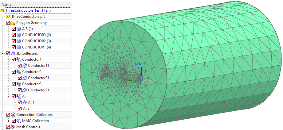
1. Change the displayed part to the Fem file.

2. Create mesh mating conditions. There should be 12 such conditions created. Blank the Air polygon body.

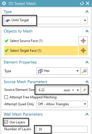
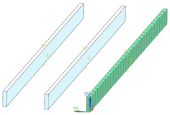
3. Mesh the ’Conductor1’ with Hexaedral elements. Use the suggested element size (6.32 mm). Activate ’Use layers’ and set the ’Number of Layers’ to 30.
   

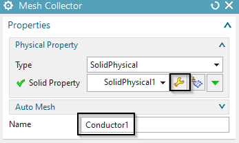
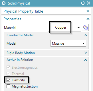
4. Edit the newly created mesh collector and his Physical. Set the material to ’Copper’ from the Magnetics material library. Check that in the setting ’Active in Solution’ the option ’Elasticity’ is on.
   

5. In the same way create meshes and Physicals for the remaining two conductors.

6. Unblank and mesh the Air body. Use tetrahedral elements and the suggested element size (129 mm). Because of the hex, tet-transition, activate the option ’Transition with Pyramid Elements’.

7. For the Air mesh, create a ’FluidPhysical’ and material ’Air’ from the Magnetics material library.

8. Select the button ’Rename Meshes and Physicals by Collectors’ from toolbar ’Magnetics’ . All meshes and Physicals will be renamed and post processing will be simplified.

EM Loads Setup - DC, AC, Short Circuit

1. Change to the Sim file.

2. Blank the 3D Collectors for easier selection. Activate (double click) the ’MagStaDC_ElasSta’ solution.

3. Create a constraint of type ’Flux tangent (zero a-Pot)’ on all 9 outside faces. Also the 6 electrode faces of the 3 conductors must belong to this group. This constraint must be used in all solutions, so drag-drop it into the others.

4. Create a Voltage load: Set the type to ’On Solid Face’, key in 0 V and select the 3 electrode faces of the 3 conductors (no matter which side). This voltage load must be active in all solutions (all but the frequency solution), so drag-drop it into the such. For the frequency solution, create a separate one in the same way.

5. In the active solution ’MagStaDC_ElasSta’, create three ’Current’ loads as follows:

   • Set the type to ’On Solid Face’ and the ’Method’ to ’Harmonic’.

   • For ’Electric Current Amplitude’ key in 50000 A, for ’Frequency’ 50 Hz and for ’Phase Shift’ 0 degrees.

   • Select the electrode face of conductor 1. Click OK.

   • Create a similar load on the second conductor with a ’Phase Shift’ 120 degrees.

   • Create a similar load on the third conductor with a ’Phase Shift’ 240 degrees.

6. Activate solution ’MagDynFreqAC50Hz_ElaSta’ and create three ’Current’ loads as follows:

   • Set the type to ’On Solid Face’ and the ’Definition’ to ’Amplitude/Phase’.

   • For ’Electric Current Amplitude’ key in 50000 A and for ’Phase Shift’ 0 degrees.

   • Select the electrode face of conductor 1. Click OK.

   • Create a similar load on conductor 2 with a ’Phase Shift’ 120 degrees.

   • Create a similar load on conductor 3 with a ’Phase Shift’ 240 degrees.

7. Activate solution ’MagDynTrans_ShortCircuit’ and create three ’Current’ loads with analytical formulas to describe the exponential behaviour of a short circuit as follows:

   • Set the type to ’On Solid Face’ and the ’Method’ to ’Analytic’.

   • Key in the following formula:
     Sqrt[2]*2e4*(Sin[2*Pi*50*$Time-1.57]+Exp[-$Time/0.0455]*Sin[1.57])

   • notice the ’1.57’ that appears two times: This describes the phase shift for the 3 phase current system.

   • Create a second and a third Current load on the electrodes faces of the second and third conductors. On the second, use a phase shift of 1.57+2*Pi/3 and on the third use 1.57+4*Pi/3

   • Drag-drop these three analytical loads into solution ’MagDynTrans_ShortCircuit_BiDir’.

Elasticity Constraints Setup

1. Activate (double click) the ’MagStaDC_ElasSta’ solution.

2. Create a ’EM Elasticity Constraint’ on the first conductor. Set the type to ’On Edges’ and select the shown two edges. Set all ’Degrees of Freedom’ to ’Fixed’ and click OK.
   

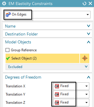
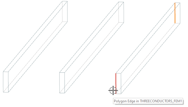
3. For the remaining two conductors, create constraints in the same way.

4. Drag-drop the three elasticity constraints into all other solutions.

Solution: EM Static, Elasticity Static

1. Activate solution ’MagStaDC_ElasSta’.

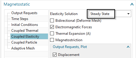
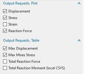
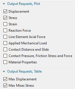
2. In register ’Output Requests’ activate results as desired.

3. In register ’Coupled Elasticity’, set the ’Elasticity Solution’ to ’Steady State’ and activate the ’Output Requests’ as shown in the picture below.
   

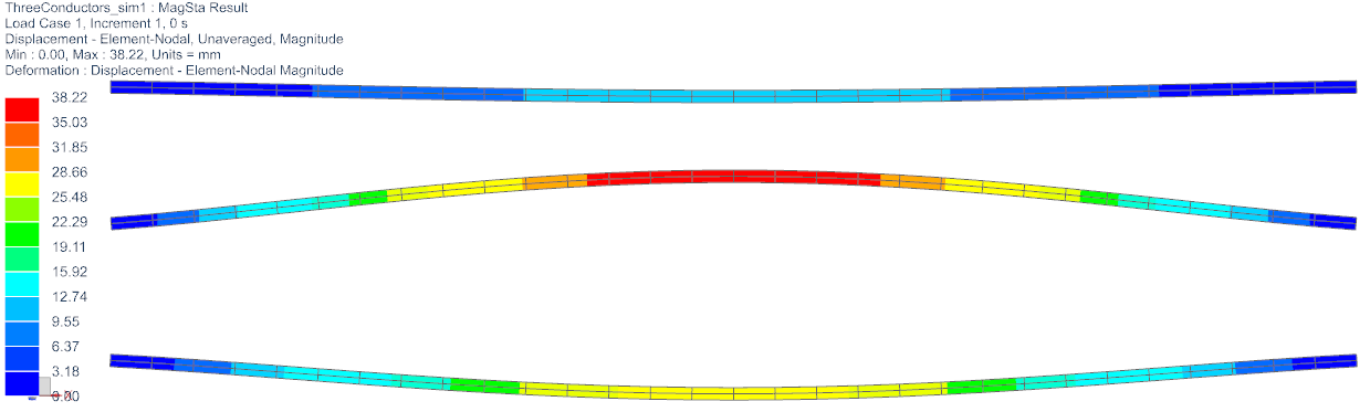
4. Solve the solution.

5. Display the Y displacement results. The maximum is 38 mm.
   

Solution: EM Frequency, Elasticity Static

In frequency domain solutions all loads and results are assumed to be harmonic. So, all results oscillate between phase angle 0 (real part), angle 90 (imaginary part), 180 and 270. Therefore, also the resulting mechanical forces come out as oscillating. To use the forces in the following elasticity solution, they are evaluated at phase angle 0.

1. Activate solution ’MagDynFreqAC50Hz_ElaSta’.

2. In register ’Output Requests’ activate results as desired.

3. In register ’Coupled Elasticity’, set the ’Elasticity Solution’ to ’Steady State’ and activate the ’Output Requests’ as shown in the picture below.
   

4. Solve the solution.

5. Check the resulting Y displacements. They should be very near to those from the static solution. The reason is that the frequency is quite low, so results are nearly static. With higher frequencies, skin effects would increase and results would change.
   

Solution: EM Frequency, Elasticity Frequency

1. Activate solution ’MagDynFreqAC50Hz_ElaFreq’.

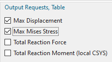
2. In register ’Output Requests’ activate results as desired.

3. In register ’Coupled Elasticity’, set the ’Elasticity Solution’ to ’Frequency Response (EM Forces harmonic)’ and activate the ’Output Requests’ as shown in the picture below.
   

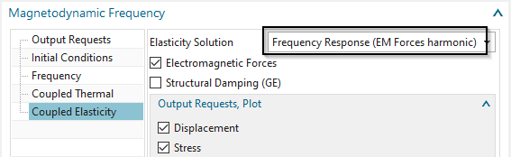
4. Solve the solution.

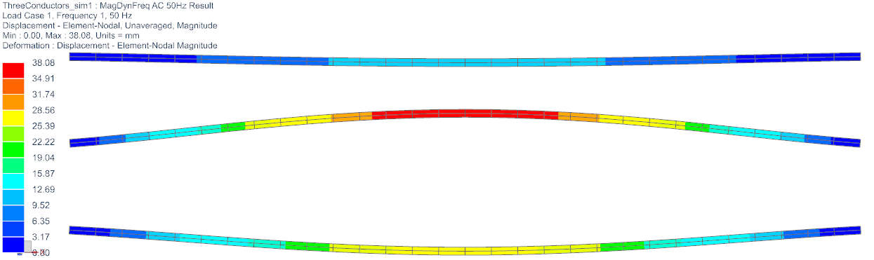
5. To check the resulting displacements, run a animation to see the oscillation. Because displacements here are complex results (frequency domain) the same rules apply as for EM results in frequency domain. To animate, set in ’Post View’, register ’Deformation’ the ’Complex Option’ to ’At Phase Angle’ and the ’Scale’ to 1, ’Absolute’. Then use the ’Animation’, set ’Style’ to ’Modal’ and ’Full cycle’, then ’Play’.
   

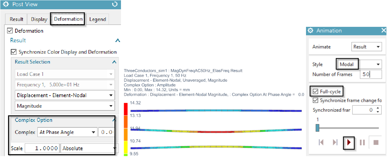
6. The maximum displacements in this simulation are about 14 mm and thus much smaller than in the previous simulation, where we had 38 mm. A reason for this can be that the excitation frequency 50 Hz is away from the mechanical natural frequency of this conductor system. Such natural frequency can by found by a solve with NX Nastran solution 103. A nice additional training would be to find that natural frequency, apply the AC load at that frequency and find the displacements then again.

Solution: EM Transient Short Circuit, Elasticity Transient

For the following two transient solutions we want to use a trick: We include the air body into the elasticity solution. By that way the air mesh will deform smoothly, forced by the conductors deformations. This trick leads to a nice air mesh at each time step even if large deformations appear (only the bidirectional solution is affected by this and thus, we could activate that only here). Of course, the air material needs as material properties a small value for Youngs modulus, Poisson ratio and Mass density. The very small Youngs modulus leads to deformations, but nearly no stresses in the air, so the conductor deformations are nearly not affected by this. As a disadvantage, solve time and memory consumption will increase, because of many more elements in the elasticity system.

1. Make the Fem part active.

2. Edit the Physical of the air and at ’Active in Solution’, activate ’Elasticity’.
   

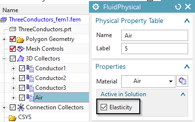
3. Optionally check that the air material has said mechanical properties.

4. Make the Sim part active again.

Following we activate the elasticity solution:

1. Activate solution ’MagDynTrans_ShortCircuit’.

2. In register ’Output Requests’ activate results as desired.

3. In register ’Time Steps’, set the ’Time Increment’ to 0.05/25 and the ’Number of Time Steps’ to 25.
   

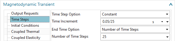
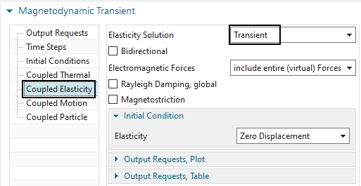
4. In register ’Coupled Elasticity’, set the ’Elasticity Solution’ to ’Transient’ and activate the ’Output Requests’ as shown in the picture below.
   

5. Solve the solution.

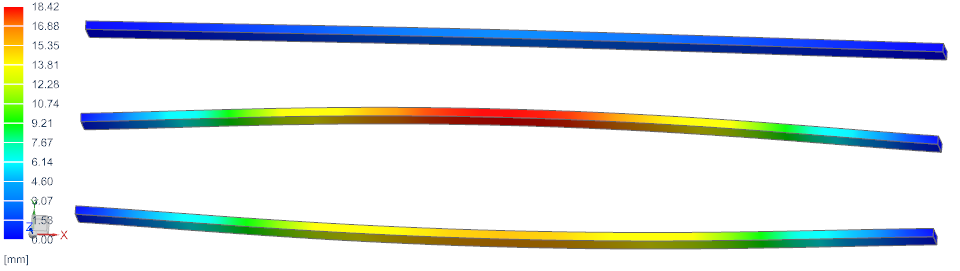
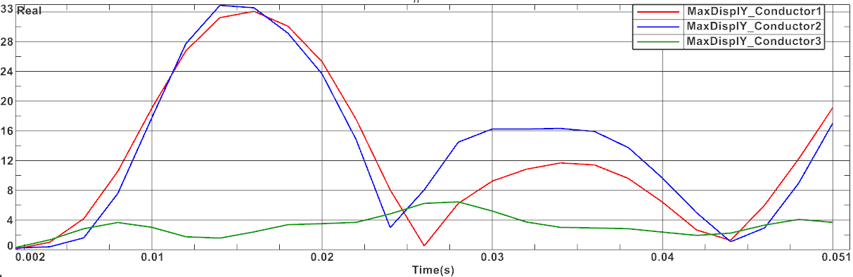
6. Display the three graphs showing the maximum conductor Y displacements over time. As the following picture shows, the maximum displacement is found at conductor 2 with about 33 mm.
   

Solution: EM Transient Short Circuit, Elasticity Transient, Bidirectional

We want to use the same settings as in the prior solution except one setting: The Bidirectional option will be active here.

1. Activate solution ’MagDynTrans_ShortCircuit_BiDir’.

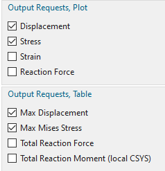
2. In register ’Output Requests’ activate results as desired.

3. In register ’Time Steps’, set the ’Time Increment’ to 0.05/25 and the ’Number of Time Steps’ to 25.

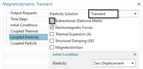
4. In register ’Coupled Elasticity’, set the ’Elasticity Solution’ to ’Transient’. Activate ’Bidirectional (Deforme Mesh)’. Also activate the ’Output Requests’ as shown in the picture below.
   

5. Solve the solution.

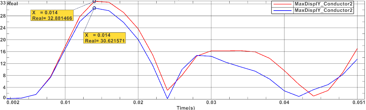
6. Display the maximum Y conductor displacements of conductor 2 of both Short Circuit solutions. As the following picture shows, the bidirectional solution shows slightly smaller displacements.
   

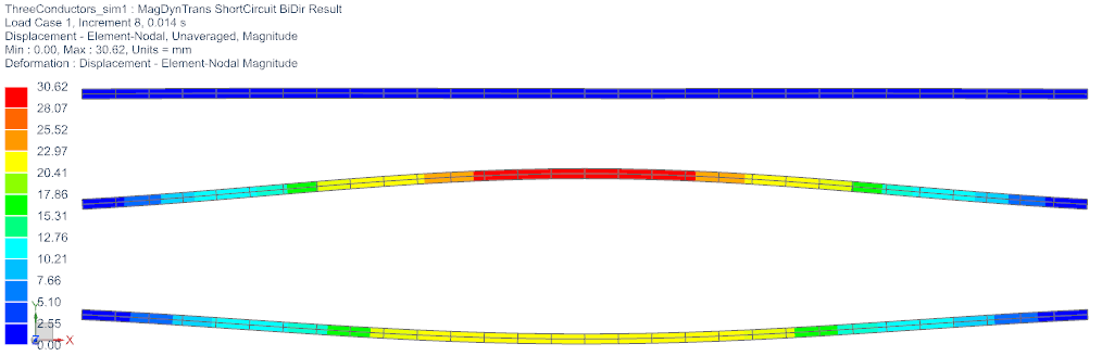
7. Display the displacements at time 0.014 (maximum, as seen above). Because in this simulation the bidirectional effect is active, now both effects are captured:

   • The EM field increases the deformation,

   • The increased distance leads to smaller EM fields.

   The solution is more realistic: The distance between conductors 1 and 2 increases, but therefore the fields become smaller and this again leads to a smaller distance.
   

The tutorial is finished.