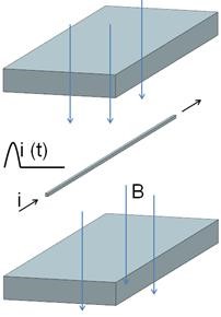
In this example we want to analyse for the elastic deformations that
result from magnetic forces. A conductor is positioned in a magnetic
field resulting from two permanent magnets. For checking purposes we
first create a static solution and compare the Lorentz forces against
theory.
In a time domain analysis we assign a half sinus current running through
the conductor and solve for the Lorentz forces that result. The Lorentz
forces on the conductor are computed for every time step and can be post
processed as graph or plot.
There follows a transient dynamic elasticity analysis to find the
conductors deformations, stresses and reaction forces. First we use the
internal elasticity solver that is delivered with Simcenter/NX
Magnetics. Because the solver is internally this process is very easy.
Alternatively to the internal elasticity solver we also want to solve by
Simcenter/NX Nastran. We apply fixed boundary conditions and import a
file that contains the Lorentz forces. As result we get deformations and
stresses.
Estimated time: 1.5 h.
Follow the steps:
download and unzip the model files for this tutorial from the
following link:
https://www.magnetics.de/downloads/Tutorials/8.CouplStructural/8.1DeformingConductor.zip
Start Simcenter, click Open ![]() and navigate to folder ’start’. Select
the file ’DeformingConductor.prt’ and click OK.
and navigate to folder ’start’. Select
the file ’DeformingConductor.prt’ and click OK.
Start application Pre/Post, Create a ’New Fem and Simulation’,
use Solver MAGNETICS and Analysis Type ’3D Electromagnetics’. Switch off
the ’Create Idealized Part’.
Hint: Because of the simple geometry, we don’t use the ’Non-Manifold’
method, so that we can take advatage of the hex elements, which enable
precise results.
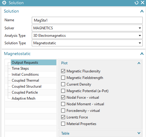
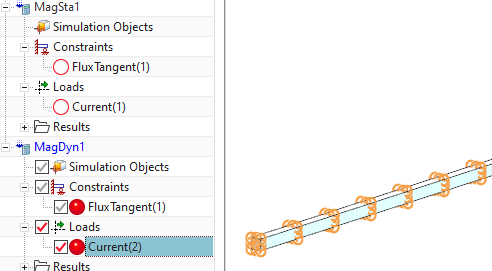
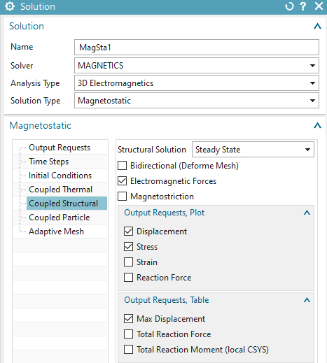
Create a first Solution of Type ’Magnetostatics’ and name it ’MagSta1’. (For checking purposes we first create a static solution.)
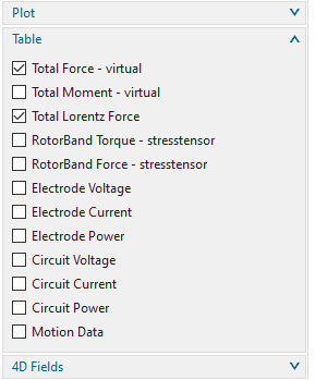
In the Output Requests under box ’Plot’ activate ’Nodal Force -
virtual’ and ’Lorentz Force’ and under box ’Table’ activate ’Total Force
- virtual’ and ’Total Lorentz Force’. You can also activate other types
you are interested in. Click Apply.
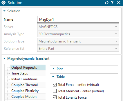
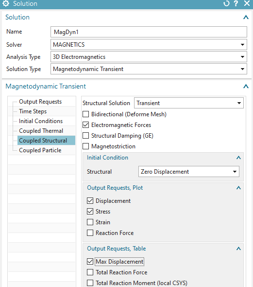
Create a second Solution of Type ’Magnetodynamic Transient’ and name it ’MagDyn1’.
Activate again the ’Plot’ output requests ’Nodal Force - virtual’ and ’Lorentz Force’. This is for viewing the forces in the plot.
Additionally activate again in the ’Table’ box ’Total Force - virtual’ and ’Total Lorentz Force’
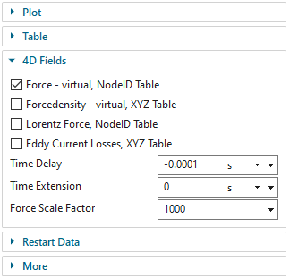
and in box ’4D Fields’ also activate ’Force-virtual, NodeID Table’. Here, at ’Time Delay’ insert -0.0001 s. This setting will shift the magnetic forces by one time step. This way Nastran will activate the forces at the same time as Magnetics does.
Additionally, key in the value 1000 into the field ’Force Scale
Factor’ because the forces must be converted from standard SI units to
mN for further use in Simcenter as input.
Hint: The virtual energy method is a more complete analysis of forces since it also captures reluctance forces and those forces that result from permanent magnets. Such are not included in Lorentz forces, because Lorentz forces compute the vector product of electric current and magnetic flux density.
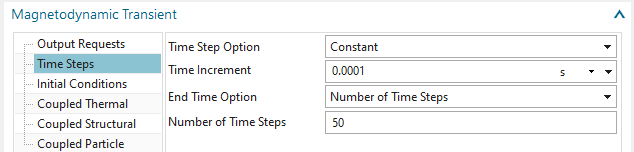
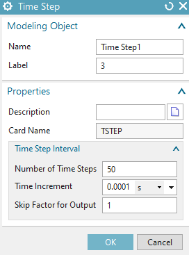
In the Time Steps you set the ’Number of Time Steps’ to 50 and
the ’Time Increment’ to 0.0001 s.
Hint: The conductor has a natural frequency at 235 Hz. You can check this by a NX Nastran Solution 103. Because 1/235Hz = 0.004s our current will force the conductor to vibrate in natural frequency.
Click OK
Switch to the Fem file
Create automatic mesh mating conditions. There should be 16 conditions created.
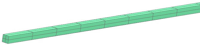
Mesh the conductor using hex elements. (Tet elements also work).
Choose the suggested element size divided by 2, and 30 layers. Prior to
meshing, set mesh controls on the four edges and force the mesh to
include four elements in the section of the conductor (see picture
below).
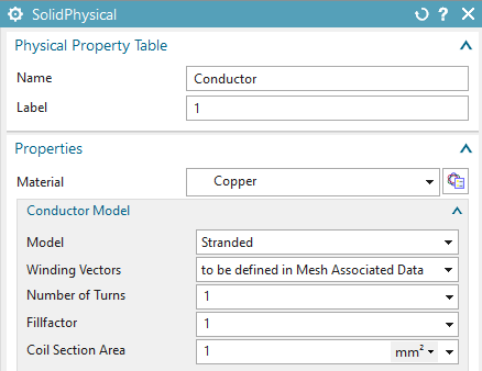
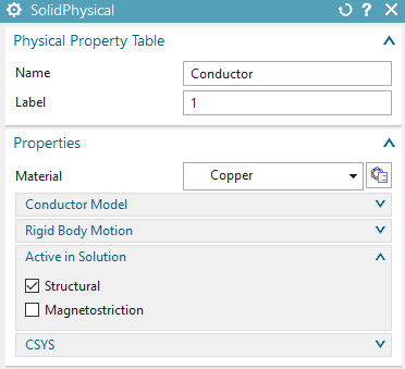
Name the mesh collector ’Conductor’ and assign material ’Copper’
from the library to the conductor. Set the ’Conductor Model’ to
’Stranded’ and use the settings as shown in the picture.
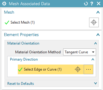
Edit the ’Mesh Associated Data’ of the conductor mesh and apply
the direction of the windings. Select one of the edges of the conductor
for this. Optionally press the ’Preview’ button to see arrows pointing
in positive current direction.
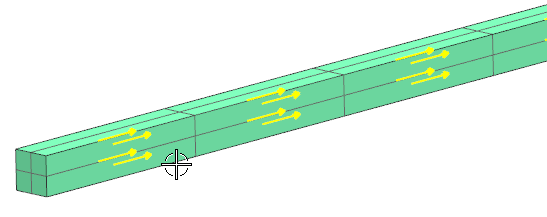
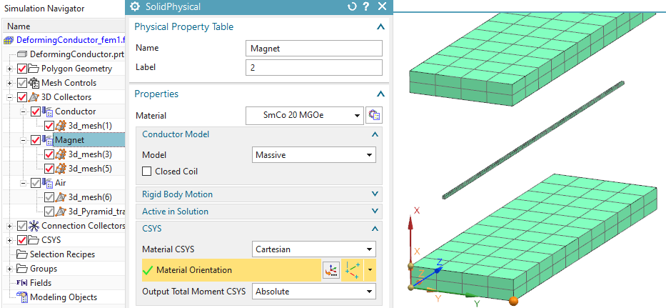
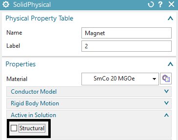
Mesh the two magnets using hex elements (Others work too).
Apply the material ’SmCo 20 MGOe’. This can be found in the material list in the NX installation folder.
Set the Magnet CSYS to Cartesian and let the X direction of it
point as shown in the below picture.
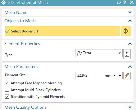
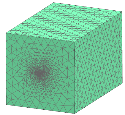
Mesh the air volume using tets and the half of the suggested
element size. Apply the button ’Transition with Pyramid Elements’ if you
used hex before.
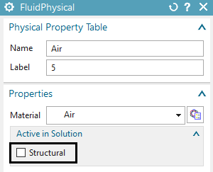
Apply a ’FluidPhysical’ and ’Air’ material to this mesh collector.
Because we want to exclude from the force computation all bodies but the conductor we must check the id labels of the Magnets physicals. We find they have id 2. We will use this in a following step in the Sim file.
Select the button ’Rename Meshes and Physicals by Collectors’
from toolbar ’Magnetics’ ![]() . All meshes and Physicals will be
renamed and post processing will be simplified.
. All meshes and Physicals will be
renamed and post processing will be simplified.
Switch to the Sim file.
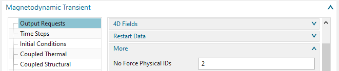
Edit solution ’MagDyn1’, in register ’Output Requests’ box ’More’
at ’No Force Physical IDs’ assign 2 because we do not want force results
on the magnets.
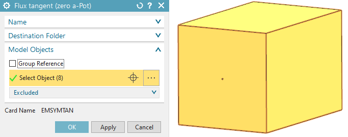
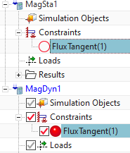
Create a constraint ’Flux tangent (zero a-Pot)’ on all 6 faces of
the air volume. Also apply this to the two small electrode faces of the
conductor. Apply this constraint to both solutions.
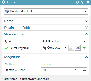
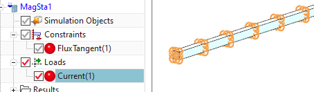
Activate the static solution and
Create a load of type ’Current’, use the default type ’On Stranded
Coil’. Select the Conductor physical. Insert an ’Electric Current’ of
100 A.
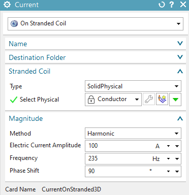
Activate the dynamic solution and
Create a load of type ’Current’, use the default type ’On Stranded
Coil’. Select the Conductor physical and set the ’Method’ to ’Harmonic’.
Insert an ’Electric Current’ of 100 A, a ’Frequency’ of 235 Hz
(remember, this is near the natural frequency) and a Phase Shift of 90
deg. (The Phase Shift changes the default cosines type load to
sinus).
Solve both solutions
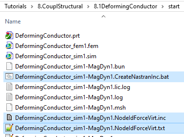
Notice that after the dynamic solution has completed, there is a new text file ’DeformingConductor1_sim1-MagDyn1.NodeIdForceVirt.txt’ in the working folder. This file contains the force that will later be transferred to NX Nastran elasticity analysis. Notice also there is a batch file in the same folder, named ’DeformingConductor_sim1-MagDyn1.CreateNastranInc.bat’. This batch must be executed to convert the text file into the format that can be included into Nastran.
In the working folder, double click that batch file
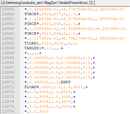
(’*.CreateNastranInc.bat’). There will be a file ’.inc’ created. This
inc file contains in Nastran syntax FORCE entries assigned to nodes and
to time steps. The DLOAD ID is set to 3000. We will later include this
file in the Nastran input file.
Postprocess the static force results.
Open the results for the static solution and display the x component of the result ’LorentzForce’. (The same can be done for the virtual forces, witch are named ’Force’. Both results are very near.)
Blank the Air mesh and all 2D meshes.
Switch from ’Contour’ to ’Arrows’.
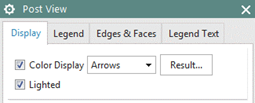
you should see a picture like below.
Hint: Depending on your current direction the direction of the force may
be flipped.
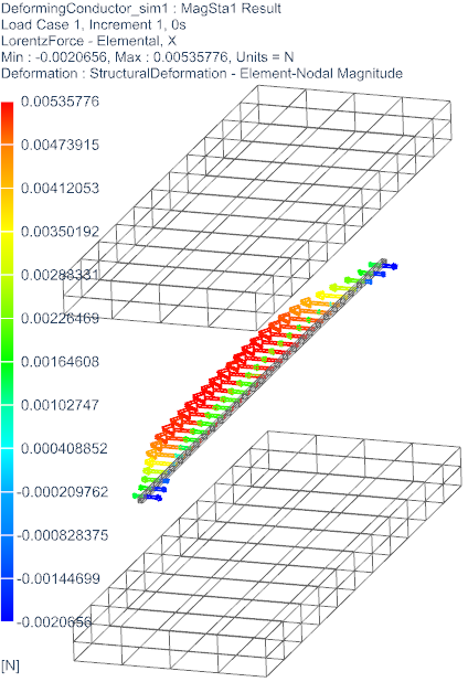
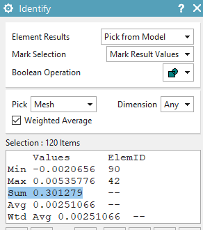
To calculate the sum of all forces acting on the conductor you
can now compute the sum of the element forces using the ’Identify
Results’ function ![]() :
:
Use the ’Identify Results’ function and set the ’Pick’ to ’Mesh’. Select the conductor mesh and find the sum is about 0.3 N.
The analytical solution for the lorentz force on the conductor
can be found as follows:
\(\overrightarrow{F_{\mathrm{L}}}=q(\vec{v}
\times \vec{B})=I(\vec{\ell} \times \vec{B})\)
with
\(I = 100 A, B = 0.03 T, \ell = 0.1
m\)
the lorentz force results to
\(F_{L} = 0.3 N\)
Though, the result from our simulation is close to this value.
Post process the dynamic solution as you like.
Save your parts. Don’t close them.
The internal elasticity solver can handle 3D and 1D elements. Tetra and hexa elements are by default solved by second order nodal shape functions. Instead of mid nodes the elasticity solver uses the element edges and faces, so result quality is high and similar to NX Nastran second order hexa and tetra elements. Also pyramids and wedges are possible, but in first order only, so be aware that these elements are not very accurate. Also there are 1D rod elements available. The solver can be used for static and transient dynamic solutions. There is no nonlinear capability available. Following we set up the deforming conductor model to use this internal elasticity solver.
Set the Fem file to the displayed part.
Edit the conductor physical. In box ’Active in Solution’ activate ’Elasticity’ (this is already activated by default).
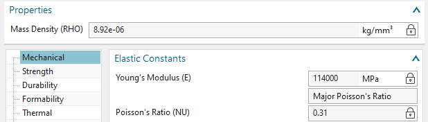
Also verify that the used material of the conductor has ’Mass
Density’, ’Young’s Modulus’ and ’Poisson Ratio’ assigned.
Check all other bodies for their setting ’Active in Solution’.
This button must be deactivated. Otherwise we would have to assign
materials and constraints to those bodies also and of course, the
simulation would require much more time, memory and disk space.
Make the Sim file to the displayed part.
Edit the static solution, in register ’Coupled Elasticity’ set the ’Elasticity Solution’ to ’Steady State’. Activate the settings as in the below picture.
Edit the transient solution, in register ’Coupled Elasticity’ set
the ’Elasticity Solution’ to ’Transient’. Activate the settings as in
the below picture.
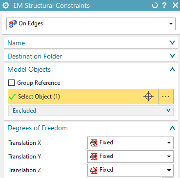
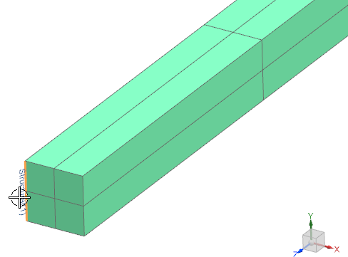
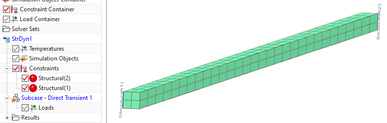
Create a constraint of type ’EM Elasticity Constraint’, set the
type to ’On Edges’ and select the two edges of the conductor as shown
below. These edges will allow the conductor to deform easily because
rotation is allowed. Set all degrees of freedom to ’Fixed’ and press
OK.
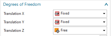
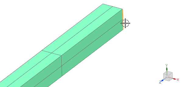
Create a second ’EM Elasticity Constraint’ on on edge of the
other side of the conductor. Fix only the x and y directions here.
Assign these two constraints to both solutions. Later we will also assign these constraints to the Nastran solution.
Solve both solutions
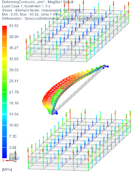
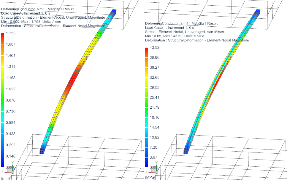
Post processing: The deformation (left) and von Mises stress
(right) result of the static solution are shown in the below
picture.
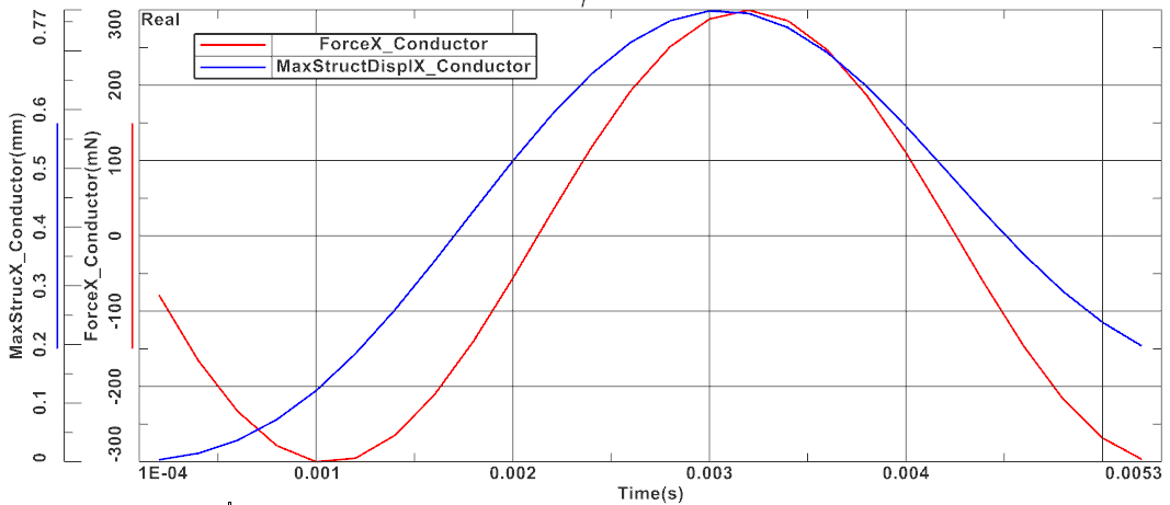
The maximum deformation over time (blue) and the force (red) from
the transient solution are shown in the picture below. Both curves are
in the AFU file, because they have been requested in the tabular output
requests of the dynamic solution.
We will now create a copy of the Fem and Sim files for the following Nastran elasticity analysis. Notice that in this analysis it is necessary to use the same node ID numbers as in the electromagnetic analysis. It is possible to add meshes. It is also possible to add mid nodes to the existing mesh for better stress results (we will do this here). Only it is not allowed to remove nodes or elements. In this case we will use a Nastran solution 109 to include transient dynamical effects. Other Nastran solution types would also work corresponding to their capabilities. The results will match with those from the previous section where the internal elasticity solver of Magnetics was used. The advantage of using Nastran is in many additional functions (contact, nonlinear materials, ...) that Nastran can handle.
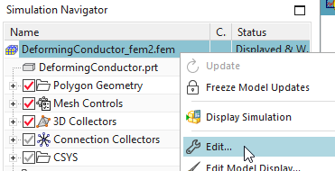
Make a copy of the Fem and Sim files. Therefore, first save the files,
then set the Fem file to the displayed part,
Do a ’Save As’ and assign the name ’DeformingConductor_fem2.fem’
The system also asks for a new Sim file. Key in ’DeformingConductor_sim2.sim’.
A ’Save As’ window appears. Press ’Yes’.
In the Fem file:
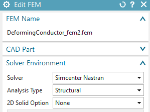
Edit the FEM file and set the Solver to NX/Simcenter Nastran,
OK.
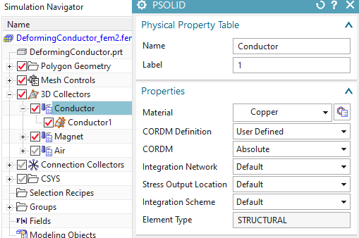
Edit the physical property of the conductor. Notice that the type
of property automatically has changed to PSOLID, because you switched to
Nastran. The material ’Copper’ is still there and since this material
has youngs modulus, poisson ratio and density available, it is valid
also for this solver.
Delete all other 3D meshes for this elasticity analysis.
Hint: This deleting is not absolutely necessary since the solver would
accept the meshes.
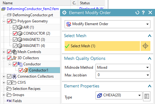
We want to use the similar shape functions in Nastran and
Magnetics. Therefore, change the mesh to Hex20: Use the function ’Order’
and use the type ’Element Modify Order’ from toolbar ’Nodes and
Elements’ and set the mesh to Hex20.
Hint: Remember, it is possible to add nodes to the model. But it is not
allowed to change the numbers of the existing nodes on which we have
computed forces and which are written into the include file.
Switch to the Sim file.
Optionally delete the two existing solutions ’MagSta1’ and ’MagDyn1’ and also the old loads. Keep the constraints because we can use them here.
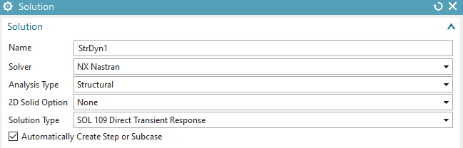
Create a new solution of type 109 with solver Simcenter Nastran
and name it ’StrDyn1’, (other transient NX Nastran solution types are
also possible) Click ’Create’ then OK. Click ’Create’ again.
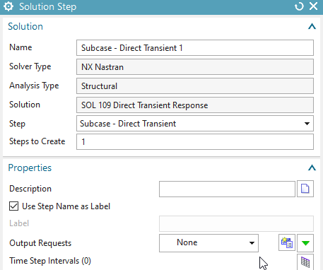
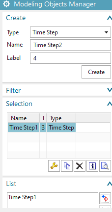
In the following dialogue ’Solution Step’ click ’Create’ ![]() for ’Time Step Interval’. In the ’Modeling Solution
Manager’ click ’create’ again and set the ’Number of Time Steps’ to 50
and the ’Time Increment’ to 0.0001 s. Click OK. Add the newly created
Time Step object to the list
for ’Time Step Interval’. In the ’Modeling Solution
Manager’ click ’create’ again and set the ’Number of Time Steps’ to 50
and the ’Time Increment’ to 0.0001 s. Click OK. Add the newly created
Time Step object to the list ![]() . Click Close and OK.
. Click Close and OK.
To add the magnetic forces, witch reside in the text file with extension ’inc’, proceed as follows:
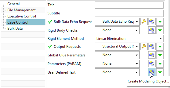
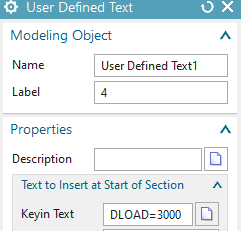
Edit the solution. In the ’Case Control’ section, create a
modeling object for ’User defined Text’. At ’Keyin Text’ insert
’DLOAD=3000’. This is the group of electromagnetic forces that will be
included.
In register ’Bulk Data’: Again create a modeling object for ’User
Defined Text’.
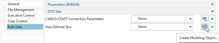 Key in the text line that points to
the include file for forces:
Key in the text line that points to
the include file for forces:
include
’DeformingConductor_sim1-MagDyn1.NodeIdForceVirt.inc’
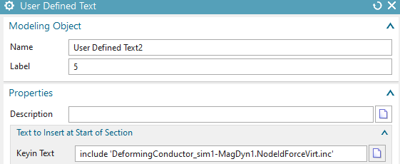
Click Ok, Ok.
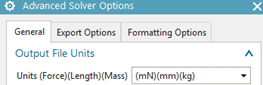
Because the force units in the include file are written in mN we
have to check that these units are used by the Nastran solution also.
Edit the Advanced Solver Options (RMB on solution) of this solution and
switch to register General. Ensure that the Output File Units are set to
(mN)(mm)(Kg).
Reuse the two constraints that were used for the electromagnetic
analysis with deformation.
Solve the solution and postprocess the results.
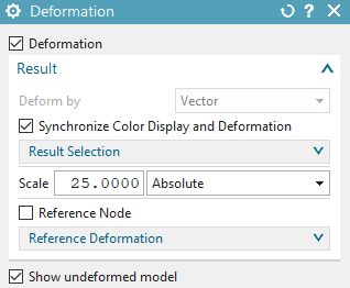
Display the displacement result of the first Increment.
Set deformation to ’Absolute’ and ’Scale’ to 25. Activate ’Show
undeformed model’
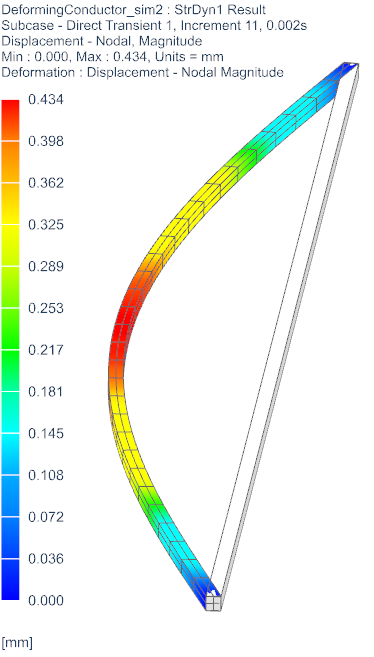
Create an animation over the iterations. It should be seen a deformation that results from magnetic forces (picture below left).
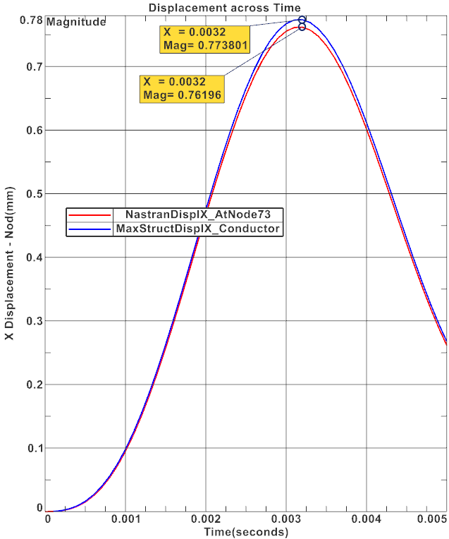
Picture below right shows a comparison of the maximum x
displacement between the Nastran (red) and the Magnetics (blue) solver
results. The deviations between the results of the two solvers are
considerably small.


Save your parts and close them.
The following described feature is available in version NX 2306
only.
Another possibility to transfer magnetic forces to Nastran uses the
total forces that are computed on each physical body. This allows the
force transfer between different models: Meshes can be different and
even 2D and 3D types can be mixed. This method has been designed to work
best with large assemblies and transient solutions in which the nastran
model contains 2D meshes while in electromagnetic 3D are present. The
process runs in the following steps:
Initial situation: The electromagnetic solution is solved with one or more bodies. The tabular forces are requested, computed and written into the afu graph file. The graph names always show the force-direction and the physical body on which it is applied. Such names are typically as ’ForceX_Conductor1’.
The user now creates a Sim and Fem file for the nastran solution. All meshes, properties can be different. Only the names of the polygon bodies in that new model must match with those names from the electromagnetic solution. In the simplest case that new model is a copy of the electromagnetic model or we simply stay in that.
The user executes the feature ’Afu-Forces to Nastran’ (found in Menu, Analyses) and will be asked for an Afu file. He assigns the one from the electromagnetic solution.
the program cycles through all graphs in that file
it checks graph names: If either ’Force’ or ’LorentzForce’ is found it extracts the force direction and the physical body name from it.
for each force, the program creates
a field from that graph.
a selection-recipe that searches for a corresponding polygon-body name. From that body all faces will be selected.
Three forces for the three directions that use the selection-recipe and the field.
all newly created forces are stored in a temporary nastran solution called ’tmp1’. From there they can be taken into the correct solution via ’drag and drop’.
The tutorial is finished.