Tutorial 5

Dipole Antenna

In this tutorial a dipole antenna is analyzed for the field patterns and for impedance and reflection coefficient. This antenna can be modeled in 2D axisymmetric or in 3D. The setup process is very similar. Following the 2D case is shown but differences for 3D there are described as hints. We walk through an existing model to explain and check the included features.

• Download the model files for this tutorial from the following link:
  https://www.magnetics.de/downloads/Tutorials/5.FullWave/5.3DipoleAntenna.zip

• Open the file DipoleAntenna1_sim1.sim. (For 3D you would open DipoleAntenna2_sim1.sim). The file already contains a complete mesh and simulation.

Meshes and Physical Properties

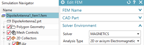
1. Change the displayed part to the Fem file.

2. Check the solver setting (right mouse button on the Fem file, Edit...). Notice, the Solver is set to ’MAGNETICS’ and the ’Analysis Type’ is ’2D or axisym Electromagnetics’. (For the 3D case the ’Analysis Type’ is 3D) Click ’OK’.
   

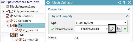
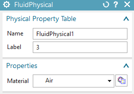
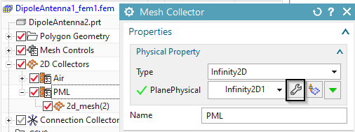
3. Edit the mesh collector ’Air’. Check that it contains a usual physical of type ’FluidPhysical’ with material ’Air’.
   

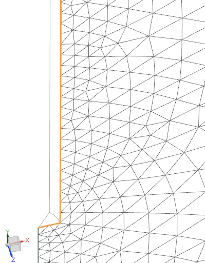
4. Next edit the mesh collector named ’PML’. It contains a border mesh around the air and a physical to describes a ’Perfectly Matched Layer’ (PML). Such PML technology is used to damp any reflection of EM waves at the outside border of the air mesh. They model a material layer, that is perfectly adapted to a given forcing frequency. If no PML would be used, all outgoing waves would reflect at the border and come back again. For the PML a physical of type ’Infinity2D’ is used. (For 3D this is Infinity3D). Check its properties as shown in the following picture.
   

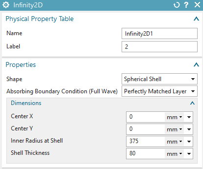
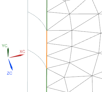
5. The PLM physical contains the following data.

   • ’Shape’: This defines the geometry type of the border mesh. It can be ’Spherical Shell’ or ’Rectangular Shell’.

   • The ’Center’ coordinates of the sphere or rectangle.

   • The ’Inner Radius at Shell’ and the ’Shell Thickness’.

Sim File Entities

1. Set the displayed part to the Sim file.

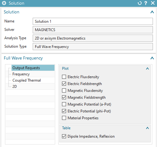
2. Edit and check the existing solution ’Solution 1’. Notice, it is of type ’Full Wave Frequency’. Set the settings for the solution as shown in the following pictures.

3. Check register ’Output Requests’:
   

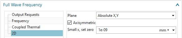
4. And register ’2D’: (This is not necessary in 3D)
   

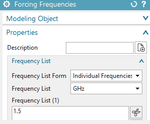
5. At ‘Forcing Frequency’:
   

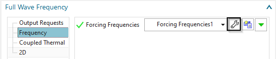
6. Click OK.

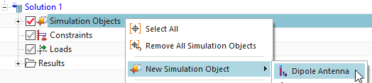
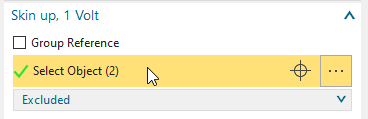
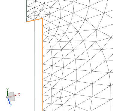
7. Edit, Check the simulation object ’DipoleAntenna(1)’. It’s of type ’Dipole Antenna’. The meaning of the three edge selections (in 3D faces) and definitions is as follows:
   

8. The ‘Skin Down, 0 Volt’: Selected are the two edges of the lower part of the dipole. Between this lower part and the following upper part there will be applied a jump in the electric field from zero to one volt. (For 3D: corresponding faces instead of edges)
   

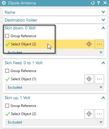
9. The ‘Skin Feed, 0 to 1 Volt’: Selected is the small edge (or corresponding face in 3D) between lower and upper part of the dipole. On this edge there will be a linear transition of the electric field.
   

10. Finally, at ‘Skin Up, 1 Volt’, the two edges (faces in 3D) for the upper part of the dipole are selected.
    

11. Box ’Feed’ differs slightly in 2D (below left) and 3D (right). In both cases there must be defined the ’Length between 0 and 1 Volt’, the gap distance. In our case this is 5 mm. In 2D there must be given the ’Direction (0V to 1V)’. Instead, in 3D, there is a ’Orientation CSYS (Origin: 0V, X Dir: 1V)’ defined, a coordinate system that points into the gap direction.
    

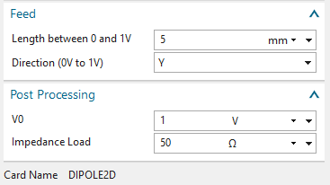
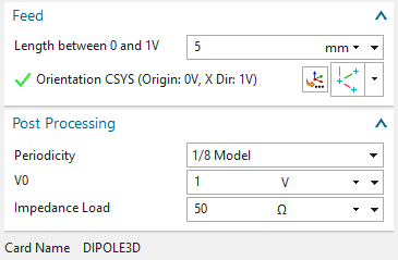
12. In the box ‘Post Processing’ there is defined ‘V0’ (the voltage jump), and the ’Impedance Load’, values that are used to compute the antenna impedance and reflection coefficient. The defaults here are ok in most cases.
    In case of 3D there is an additional option ’Periodicity’. Here we define whether the model is complete (’Full Model’) or only a part.

13. Solve the solution.

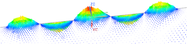
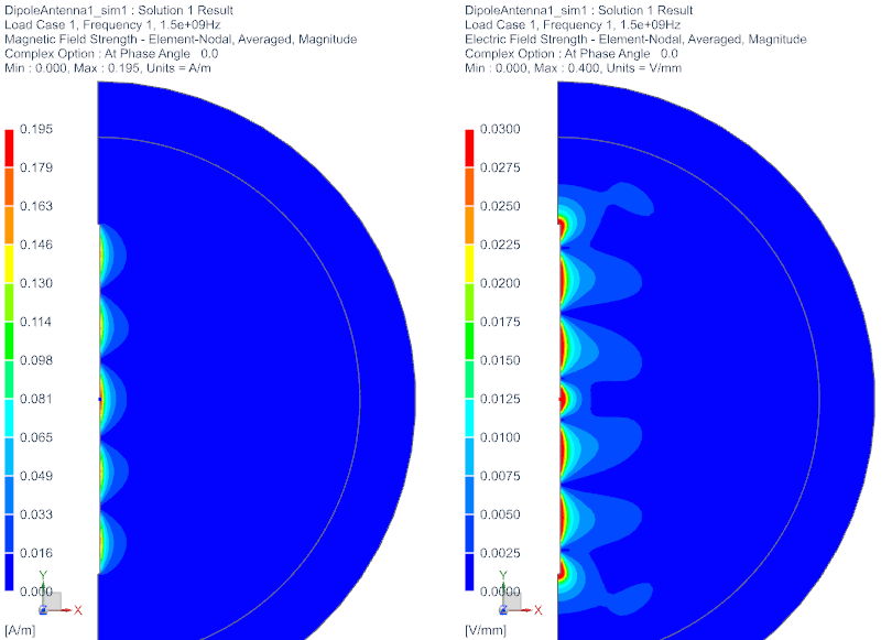
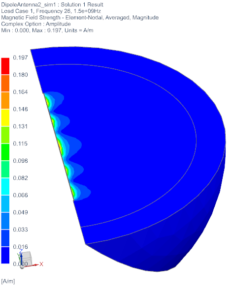
14. Post process the Results. Next picture left shows the magnetic and right the electric field strength, both with option ’At Phase Angle’, so showing the real parts.
    

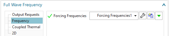
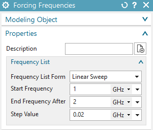
15. Next we modify the forcing frequencies to a sweep, see below picture, and solve again.
    

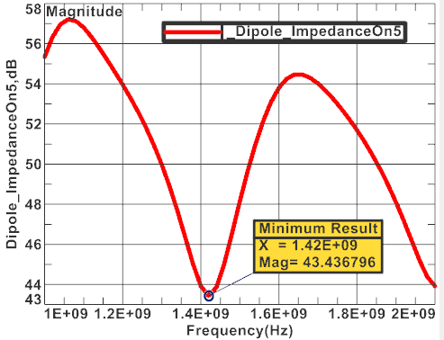
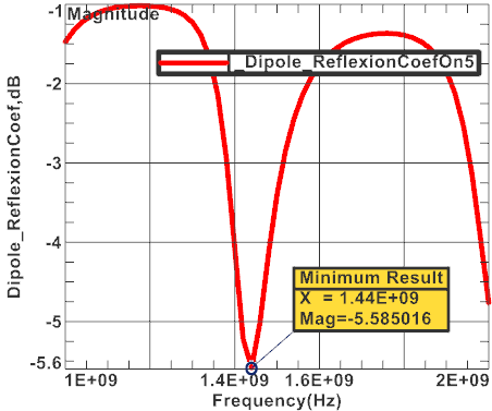
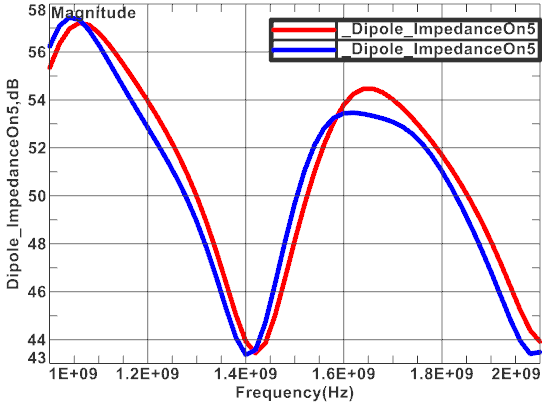
16. the resulting impedance and reflection coefficient are now graphs over the frequency as shown below (y axis set to type ’dB’). They show a minimum at about the same frequency of 1.44 GHz.
    

17. the resulting graphs from the 3D model differ slightly. Smaller mesh sizes would further reduce this difference. The following picture below right shows both 2D (red) and 3D (blue) together.
    

18. The tutorial is complete.