Tutorial 3

20 GHz Waveguide Combiner

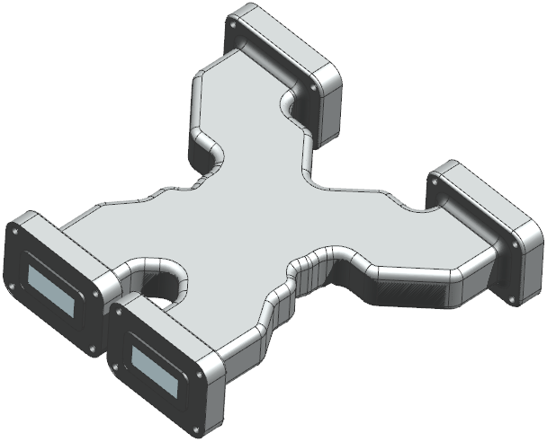
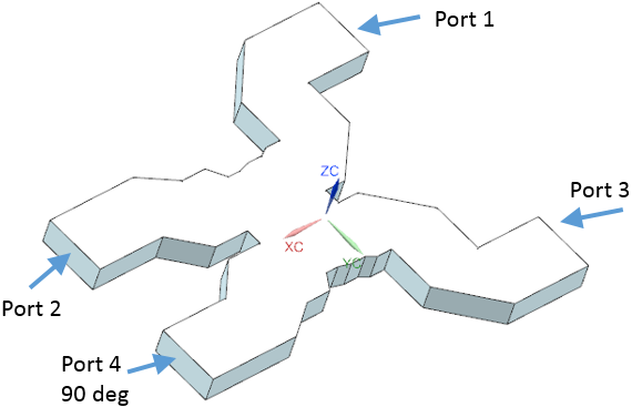
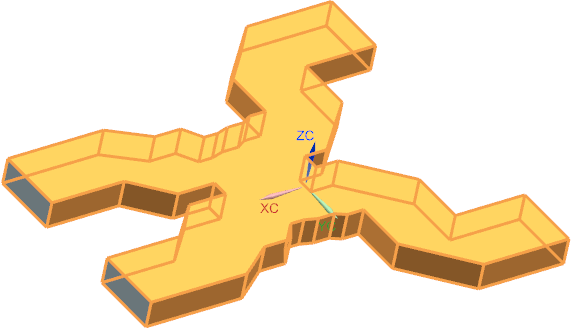
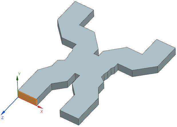
The waveguide combiner shown in this exercise is used to combine the output power of two 20 GHz power amplifiers. The two outputs of the amplifiers are fed into ports 2 and 4 of the waveguide with a 90 degree phase change. The two other Ports 1 and 3 are output ports. The phase change between the input ports leads to an absorption of the wave in one of the output ports. The problem is also described and analyzed in [Arcioni].

What you learn in this example:

• Performing a Waveguide analysis in frequency domain,

• Use of Phase changed port signals,

• Use Finite Conductivity Boundary Condition.

• Calculate s-Parameters.

Estimated time for the example: 1 h. Follow the steps:

Waveguide Solution

We first create the simulation file structure and a solution for this waveguide problem.

1. Download the model files for this tutorial from the following link:
   https://www.magnetics.de/downloads/Tutorials/5.FullWave/5.2WaveguideCombiner.zip

2. Open the part file WaveguideCombiner.prt.

3. Start the application Pre/Post.

4. Create New FEM and Simulation.

5. Select the Solver MAGNETICS and

6. Analysis Type 3D Electromagnetics.

7. Switch off idealized part.

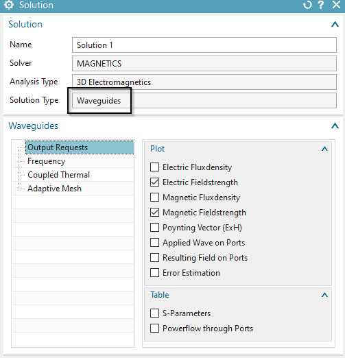
8. Select the Solution Type ’Waveguides’.

9. In register ’Output Requests’, ’Plot’ set ’Electric Fieldstrength’ and ’Magnetic Fieldstrength’ on. In a later step we will activate ’S-Parameters’.
   

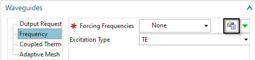
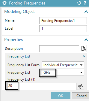
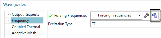
10. In register ’Frequency Domain’ create a ’Modeling Object’ for the forced frequency and set the ’Forcing Frequency’ to 20 GHz. Accept the default ’Excitation Type’ ’TE’ since we want to apply this type of wave. Click ’OK’ to finish the solution menu.
    

Meshing

Switch to the Fem file.

1. Blank the housing polygon body.

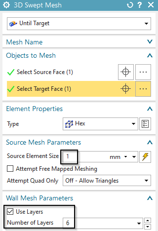
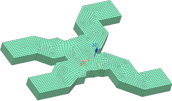
2. Mesh the air volume using hex elements. Use an element size of 1 mm and 6 layers over the thickness. Of course, tetrahedral elements would also work.
   

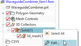
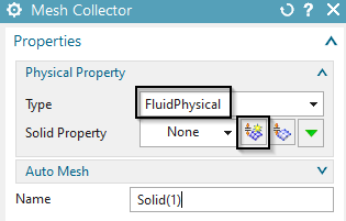
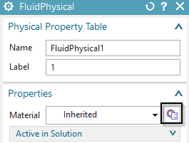
3. Assign a ’Physical Property’ of type ’FluidPhysical’ and select the material ’Air’ from the Magnetics material library.
   

Finite Conductivity Boundary Condition

We create a condition on the boundary that represents the electric conductive border material.

1. Switch to the Sim file.

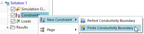
2. Create a constraint of type ’Finite Conductivity Boundary’. Select all faces but the 4 port faces.
   

3. Choose the material properties as shown in the picture. These describe a aluminium type material. The thickness of this material layer will be computed by the skin depth. That skin depth results from the given electric conductivity and the applied enforced frequency.
   

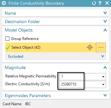
4. Click ’OK’ to create the constraint.

Wave Ports

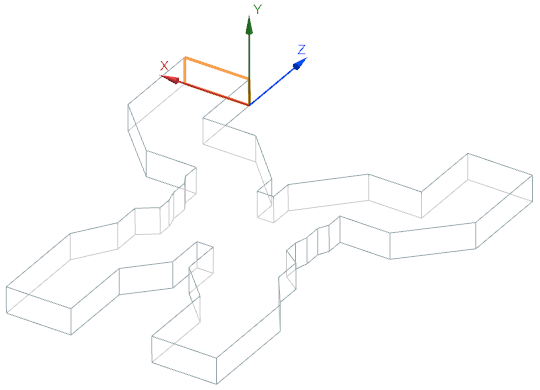
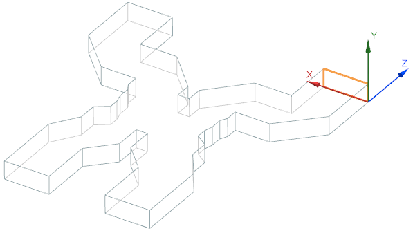
Now we create the ports at which signals are applied. These correspond to the prior picture, that is again shown here below right.

1. Define the active Wave Port number 2:

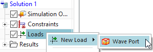
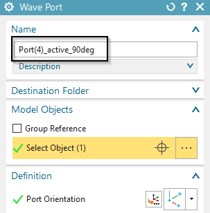
   • Create a load of type ’Wave Port’.
     

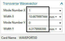
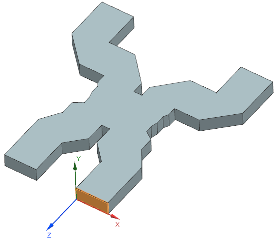
   • Select the face of port 2 and define the Port Orientation as shown in the below picture. Name this load Port(2)_active. Assign the settings as shown in the below dialog.
     

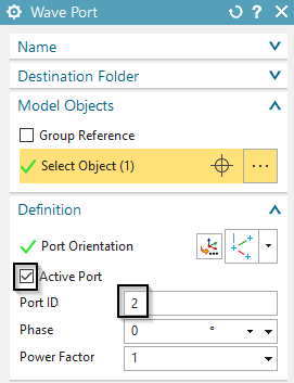
   • Click ’OK’.

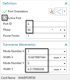
2. Define Wave Port 4

   • Create a load of type ’Wave Port’.

   • Select the face of port 4 and define the port orientation as shown in the picture.

   • Name the load ’Wave Port(4)_active_90deg’

   • Assign the similar settings as for port 2 but set the ’Phase’ to 90 deg and the ’Port ID’ to 4.
     

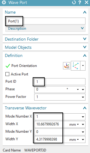
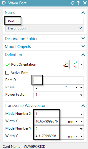
3. Define Wave Ports 1 and 3

   • Create again a load of type ’Wave Port’ (this is done two times now, for the remaining ports 1 and 3. These two get quite similar input).

   • Select the face of port 1 (picture below left) and port orientations as done already before. Do the same for port 3 (picture below right).
     

   • Name the loads Port(1) and the second one Port(3).

   • Assign the shown settings (below picture, left port 1, right port 3).
     

Solve and Postprocessing Field Results

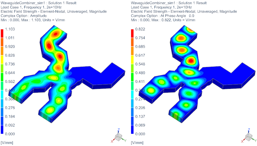
1. Solve the solution. Open the plot results and hide the 2D meshes in ’Post View’.

2. After solve has finished, display the Electric Fieldstrength. The following picture shows left the ’Amplitude’ and right the ’Signed Amplitude’ at phase 0 deg (explained below) what means the real part.
   

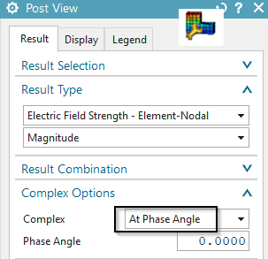
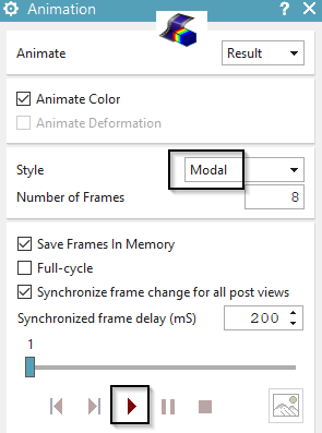
3. Animations can be used to show the complex result converted to time domain. To do so you click ’Edit Post View’, register ’Result’. Set the option ’Complex’ to ’At Phase Angle’. Then go to ’Animation’ and set the ’Style’ to ’Modal’ and click ’Play’. The animation runs over the phase angle now and that represents the time domain behaviour of this frequency result.
   

S-Parameters and Frequency Sweep

In a following solution we want to solve for the S-parameters. Also we want to perform a sweep over a frequency range to find out how the S-parameters behave at different excitation frequencies. For S-parameter calculation there must be only one active port in a solution and the results will show how the other ports interact with the active one. To find the complete matrix of all interactions, one had to run several solutions, each with another port being active.

1. Prepare the model for S-parameter calculation:

   • Clone the existing solution and rename the new one to ’SparamP2active’. In this solution we will have only port 2 active.

   • Modify the wave port 4 and set it to inactive. (Maybe create a new wave port for that or clone the old one. Otherwise you will overwrite it.)

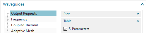
   • Edit the solution. In register ’Output Requests’, ’Table’, activate ’S-Parameters’.
     

2. Activate Frequency Sweep:

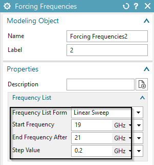
   • Edit the solution. In register ’Frequency’, create a new ’Modeling Object’ for ’Forcing Frequencies’. Set the list form to ’Linear Sweep’ and key in the values for start, end and step as shown in the below picture.
     

3. Solve the new solution ’SparamP2active’.

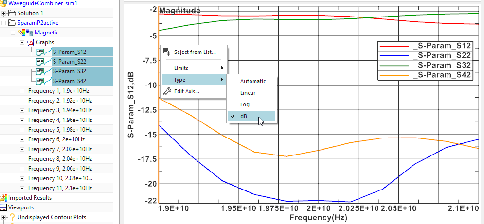
4. After solve has finished, open the tabular graph results and display the S-Parameters over Frequency. Set the Y axis type to ’dB’ to display the parameters in the usual way.
   

The tutorial is complete. Save your files and close them.