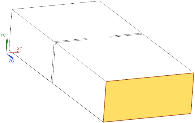
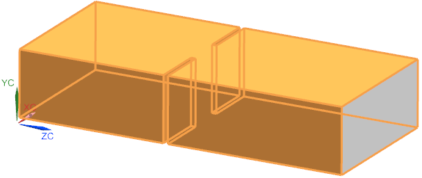
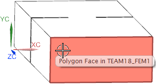
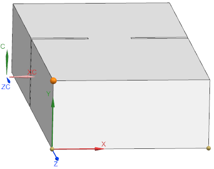
Goal of this Team benchmark example is to find the resonance frequency of a waveguide cavity. The highlighted face shall be applied by a transversal electric wave mode of type TE10 as shown in the right side of the picture. A full wave solution is necessary to analyze for resonance of such electromagnetic waves. The original task description of Team 18 can be found at [Team18task].
What you learn in this example:
Performing a 3D Full Wave analysis for Waveguides in frequency domain.
Learn how to define the basic settings for wave ports.
Estimated time for the example: 0.5 h.
For the setup of this model, follow these steps:
Download the model files for this tutorial from the following
link:
https://www.magnetics.de/downloads/Tutorials/5.FullWave/5.1Team18.zip
Open the part file Team18.prt.
Start the Pre/Post application.
Create New FEM and Simulation.
Choose Solver MAGNETICS and
Analysis Type ’3D Electromagnetics’,
switch off idealized part.
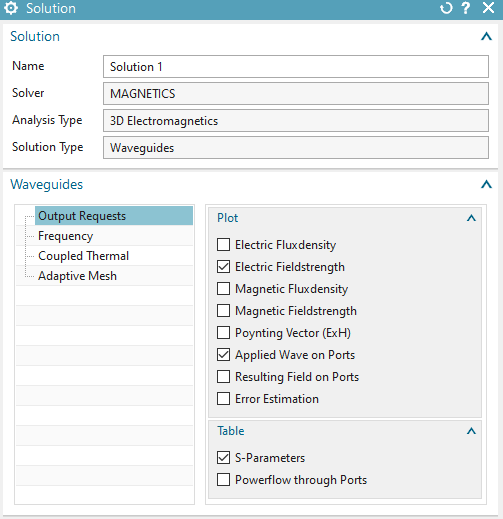
Select Solution Type ’Waveguides’.
In register ’Output Requests’, ’Plot’ set ’Electric Fieldstrength’ and ’Magnetic Fieldstrength’ on.
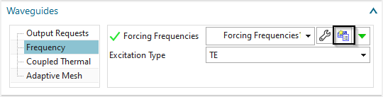
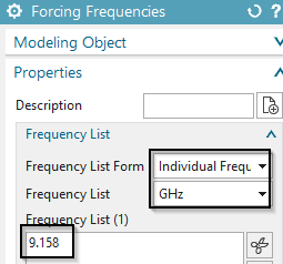
In register ’Frequency’ at "Forcing Frequency’, create a modeling object for the used frequency with 9.158 GHz (This is already the found resonance frequency). Alternatively, we could run a sweep over a frequency range to search for resonances.
in box ’Table’ activate ’S-Parameters’.
Switch to the Fem file
Blank the polygon body ‘Housing’. This body is not needed in the analysis.
Mesh the air volume using tets. Use the suggested element size divided by 4. (4.63/4 mm)
Assign material ’Air’ to it.
Switch to the Sim file.
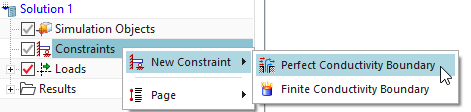
Create a constraint of type ‘Perfect Conductivity Boundary’ to
all faces but the entrance face for the incoming wave.
Next we are defining the incoming wave. We must define a TE10 wave. TE means that the electric field vector in Z direction must be zero. The opposite is true for TM waves; Here the magnetic field vector is zero in Z. For both TE and TM the first index defines the number of maxima in X direction and the second index those in Y direction. See chapter ’Summary of wavetypes for rectangular guides’ for further information.
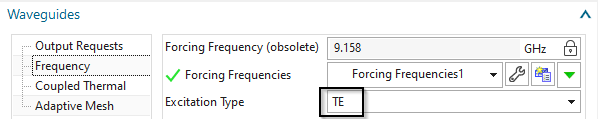
To set the type to TE, edit the solution parameters.
In register Frequency Domain set the ’Excitation Type’ to ’TE’.
(Since this is the default, there is nothing to do.)
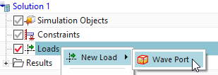
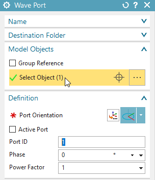
Create a load of type ‘Wave Port’
At ’Model Objects’, select the entrance face,
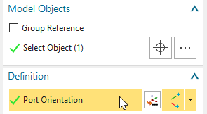
At ’Port Orientation’, use the ’CSYS Dialog’ (or any other) to
define a coordinate system. Define the center at one face corner, the x
direction along one edge and the y-direction along a perpendicular edge
of the face.
Hints: The CSYS center defines the beginning position of the incoming
wave. This position plus the ’Width X’ defines the ending position.
Between start and end the wave can have a number of maximums. This
number of maximums will be defined by the ’Mode Number X’. The
corresponding applies for Y.
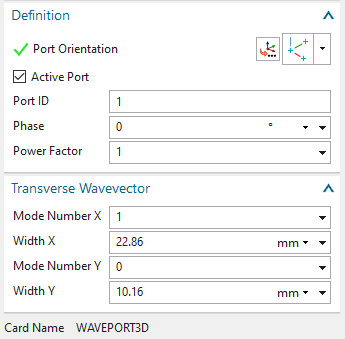
Toggle on ’Active Port’, leave ’Port ID’ as 1 and ’Phase’ as 0.
At ’Transverse Wavevector’: Set ’Mode Number X’ to 1 and ’Mode
Number Y’ to 0. This setting describes the characteristic of the desired
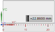
TE10 wave. For ’Width X’ and ’Width Y’ key in the full width of the CAD
face: In X direction use 22.86 mm and for Y use 10.16 mm. Of course, its
also possible to use the graphical measuring feature.
Click OK to finish the dialogue.
Solve the solution
Postprocessing:
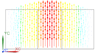
Display the electric field strength. Blank the 2D meshes under
Post View. Check the pattern of the wave. The resulting field should
show a standing wave as seen in the below picture. The maximum value of
electric field strength can vary depending on how closely you find the
resonance frequency.
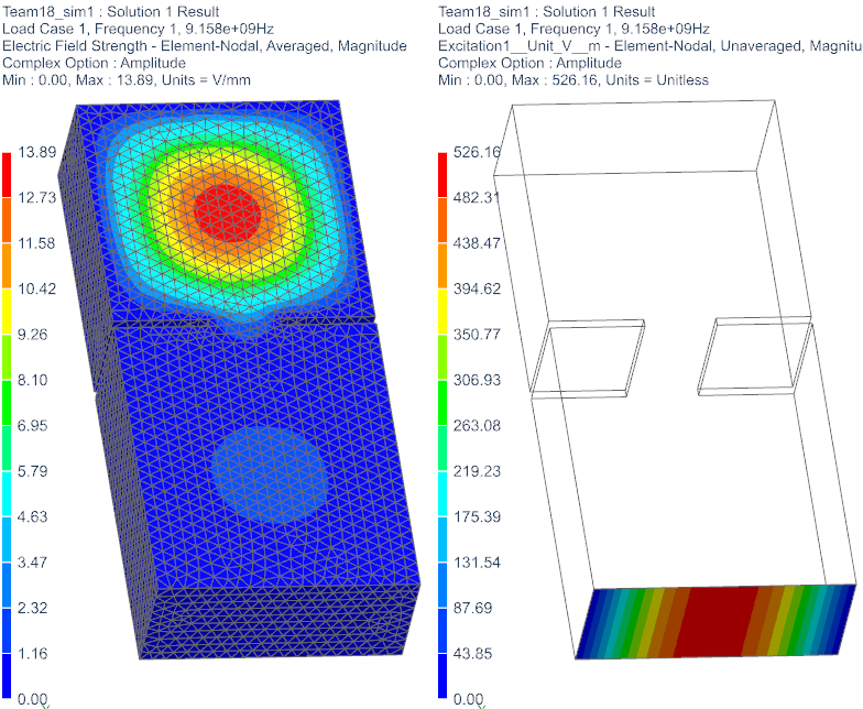
Display the ’Excitation’ result. (Picture above right.) This shows the defined TE10 wave at the port face. Check the pattern.
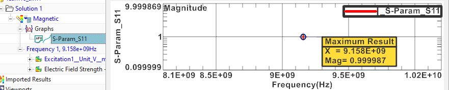
Check the calculated S-Parameter S11. It is very near to 1.
The tutorial is finished.