Additional features to be used in several solutions are demonstrated
in this chapter.
Contact Resistance -
Electrical and Thermal
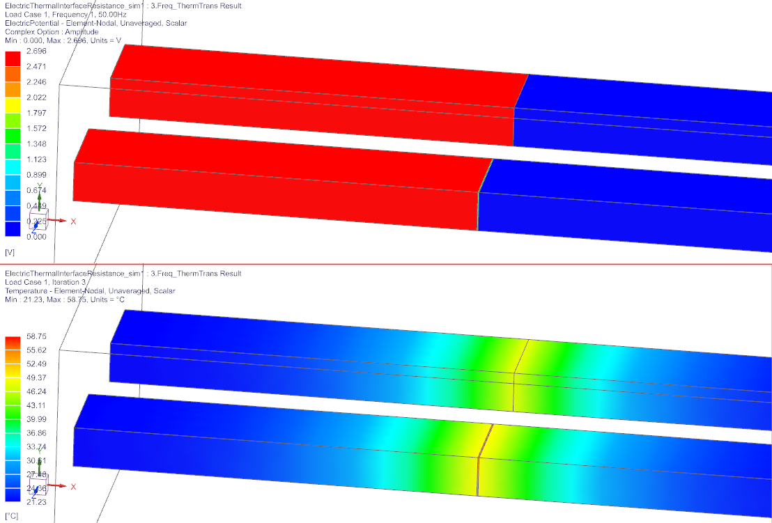
In this example we show the feature ’Contact Resistance (One
Surface)’, that can be used to model thin gaps. For comparison, the
simulation model contains two conductors with identical boundary
conditions. They differ only in the model of the gap: One has a gap with
3D elements (e.g. the conventional way) while the other uses the feature
’Contact Resistance (One Surface)’ with 2D elements at the gap. Both
results are very similar. The below picture shows the two conductors: In
front the one with 3D, behind the one with 2D elements at the gap. The
gap has 0.25 mm thickness, thus it is hardly visible. The upper shows
electric potential, the below shows temperature results.
On the left and right electrode faces there are fixed currents (100
Amps) and zero voltages applied. Different solution types are used:
DC Conduction - steady State
Magnetodynamic Frequency with coupled Thermal (Static)
Magnetodynamic Frequency with coupled Thermal
(Transient)
other solution types are also possible.
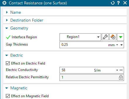
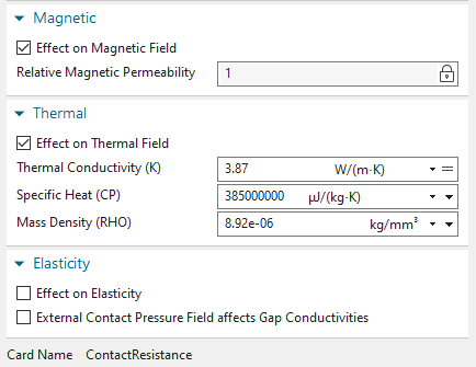
The picture also shows the dialogue of the simulation object that is
used to create such an ’Contact Resistance (One Surface)’
The text file
’ElectricThermalInterfaceResistance_sim1-1.DC.EddyCurrentLoss.txt’
contains the computed eddy current losses. It can be seen that the
losses in the 3D and those in the 2D region, are very close:
Eddy Current losses in 3D gap: 134.6982758915086 W.
Eddy Current losses in 2D gap: 134.6982758297983 W.
The tutorial is complete.
Flux
Coupling - Electrical and Thermal
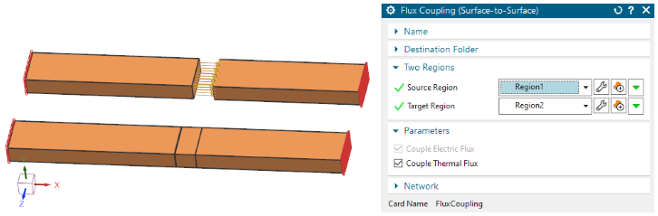
In this example we show the feature ’Flux Coupling
(Surface-to-Surface)’ that can be used to couple the flux from two
faces. Either the electric or the thermal or both fields can be coupled
and the two faces must not match or use the same nodes. The feature
creates a bidirectional circuit link between the two faces that allows
the flux to be coupled. For comparison, the sim- ulation model contains
two conductors with identical boundary conditions. They differ only in
the model of the gap: One has a gap with 3D elements (e.g. the
conventional way) while the other uses the feature ’Flux Coupling
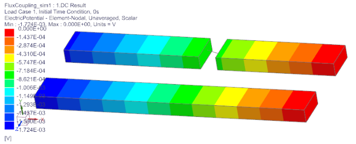
(Surface-to-Surface)’. The below picture shows the two conductors: In
front the one with 3D, behind the one with the Flux Coupling.
Download the model files for this tutorial from the following
link: https://www.magnetics.de/downloads/Tutorials/10.Features/10.7FluxCoupling.zip
There is one model (FluxCoupling_sim1.sim) with a DC and a Frequency
solution. The other model (Flux-Coupling_sim2.sim) contains also thermal
solutions and uses ’Flux Couplings’ with additional ’Contact
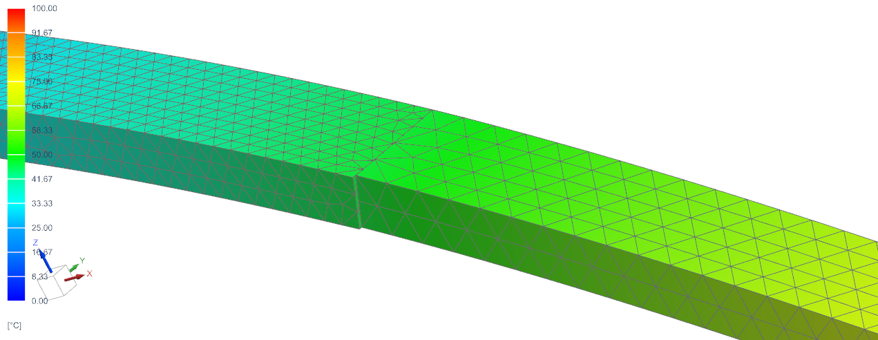
Resistance’. The following figure shows the two conductors. On the left
and right electrode faces there are fixed currents of 100 Amps and zero
voltages applied. Thus, an electric current will flow through the
conductors
The solution is a DC Conduction, but also other solution types can be
used. If the faces are inside of a fluid, be aware that the fluid must
not touch the faces. The example model shows how that can be achieved.
The picture below shows the dialogue of the simulation object that is
used to create such an ’Flux Coupling (Surface-to-Surface)’
The tutorial is complete.
Surface
to Surface Glue - Electromagnetic, Elastic and Thermal
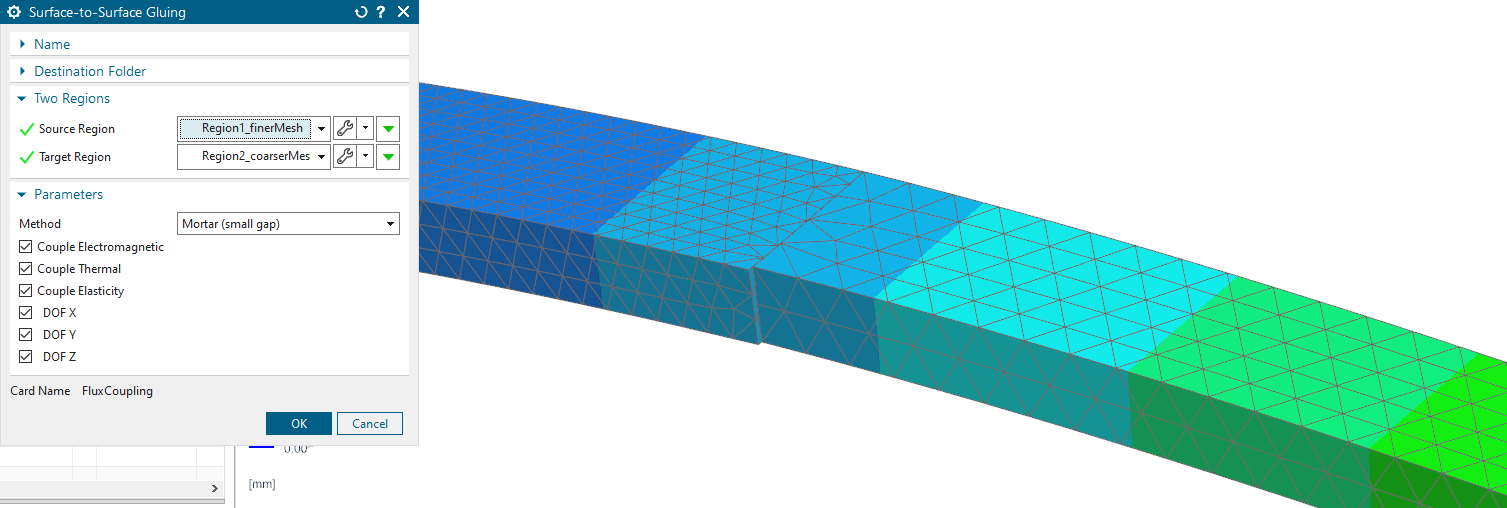
In this example we show the feature ’Surface to Surface Glue’ that
can be used to couple two faces with non-conformal mesh, e.g. with
non-matching nodes. The feature uses the mortar FEM method that allows
the faces to be coupled.
Download the model files for this tutorial from the following
link: https://www.magnetics.de/downloads/Tutorials/10.Features/10.8SurfaceSurfaceGlue.zip
There is a model (MortarGlue_sim1.sim) with a Elasticity and a Thermal
solution. The following figure shows the conductor. On the left and
right electrode faces there are fixed Temperatures of 0 and 100
deg.
The solution is a DC Conduction, but also other solution types can be
used. If the faces are inside of a fluid, be aware that the fluid must
not touch the faces. The example model shows how that can be achieved.
The picture below shows the dialogue of the simulation object that is
used to create such an ’Surface-to-Surface Glue’
The tutorial is complete.
Orthotropic
Materials Modeling
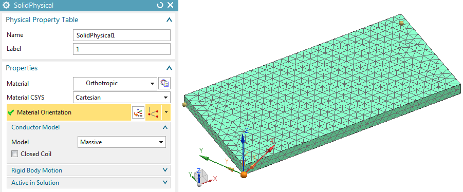
In this example electric current flows through a conductor that is
modeled with orthotropic electric conductivity.
Orthotropic Electromagnetic properties can only be used with the (old)
Magnetics material model. Thus, the custom_dirs.dat file or
alternatively, the variable UGII_USER_DIR must point to the installation
folder of Magnetics.
The following figure shows the conductor and his physical properties
menu. Notice the Material CSYS is set to Cartesian and a new coordinate
system is defined with x direction pointing diagonal across the
plate.
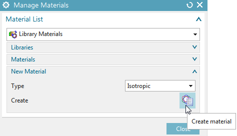
An orthotropic material is created as shown in the next picture.
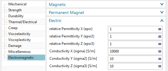
The properties of this orthotropic material are shown below. In this
case we use orthotropic electric conductivities and we set the x value
much higher than y and z.
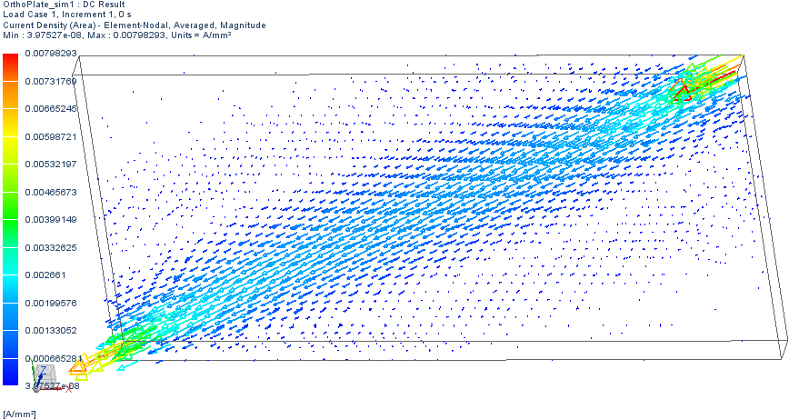
On the left and right electrode faces there are loads (one ampere left
and zero volt right) applied and a DC Conduction Steady State analysis
is performed.
The next figure shows the electric current density as it results from
this simulation.
Magnetic Hysteresis,
Jiles-Atherton Model
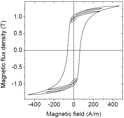
In this example we model magnetic hysteresis effects using the
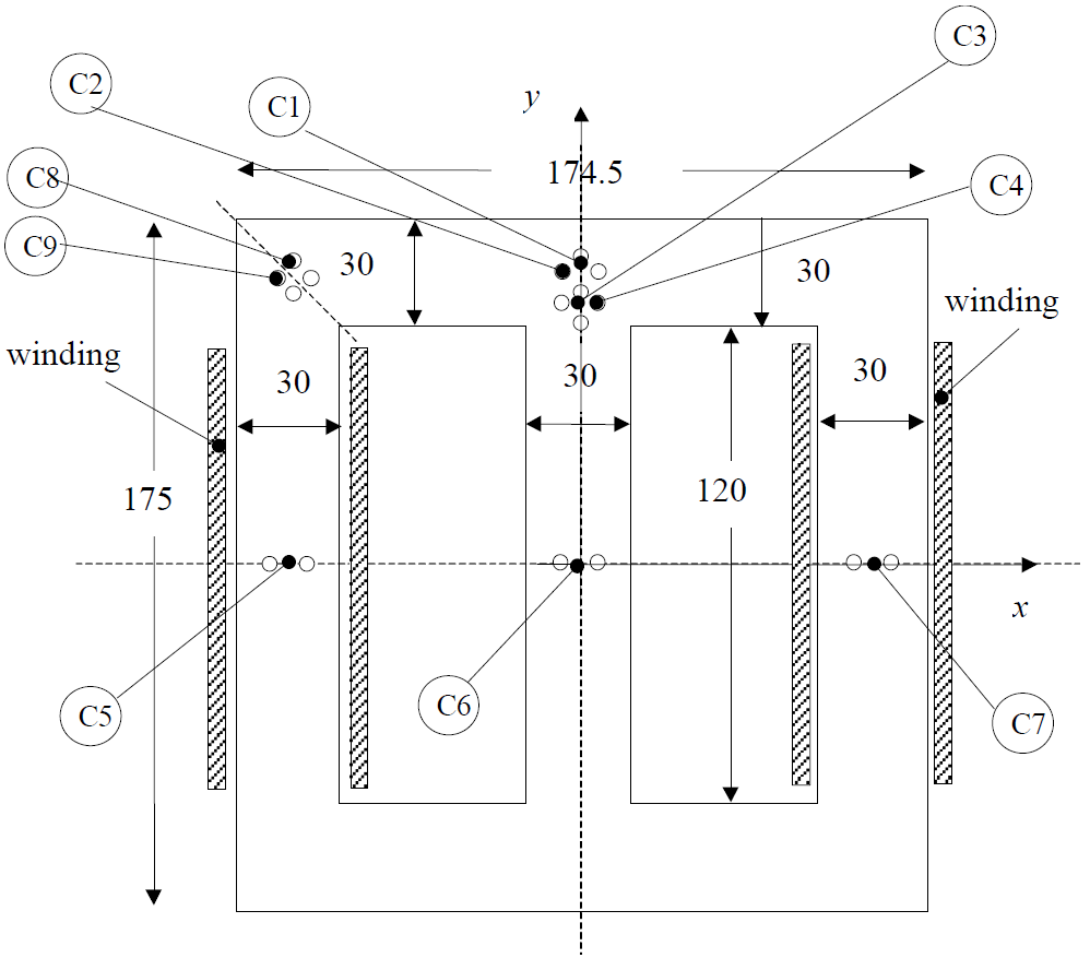
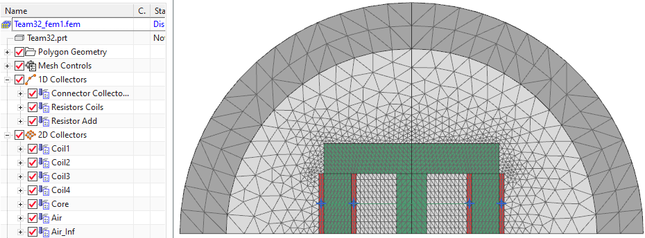
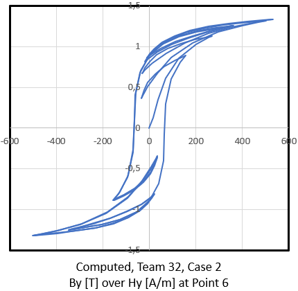
Jiles-Atherton model. The used example is the TEAM 32 test case whose
setup is shown in the below left picture. The picture right side shows
the expected hysteresis loop as it results from alternating magnetic
fields at point C6.
More background information about this test example and available
measurements can be found in the reference paper at
www.compumag.org/wp/wp-content/uploads/2018/06/problem32.pdf
The model consists of two coils and a core. In the paper there are 4
cases described. We model case 2: The two coils are connected in series.
The series is supplied by a sinusoidal voltage of 13.5 V (peak value).
Additionally there is a fifth harmonic applied with same phase.
In Simcenter, open the Sim file ’Team32_sim1.sim’.
Set the displayed part to the Fem file.
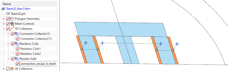
Check the existing meshes and physical properties. Notice also,
there are 1-D circuit elements included to connect the coils in series
and apply additional resistances. Two remaining coil connectors are
connected with the voltage load as seen later in the Sim file.
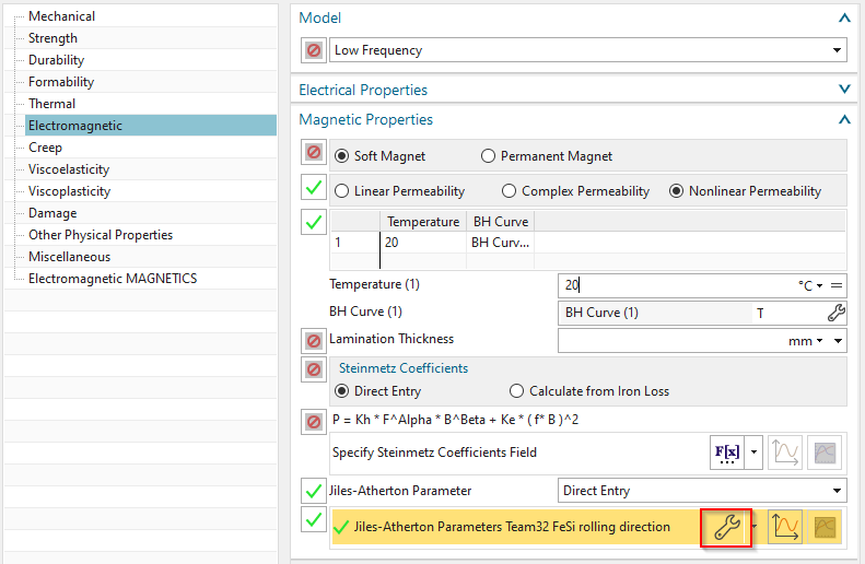
To model magnetic hysteresis by Jiles-Atherton the material
description must have Jiles-Atherton-Parameters. We check this for the
core material:
Edit the core material (t32_Core_mat_hyst) and open register
’Electromagnetic’.
At the very below of the menu, there are the definitions for
’Jiles-Atherton Parameter’. Notice, these parameters are accessible only
if in register ’Electromagnetic’ the ’Model’ is set to ’Low Frequency’
and if the ’Magnetic Properties’ are set to ’Soft Magnet’ and ’Nonlinear
Permeability’.
Click the ’Edit’ button (at very buttom of the menu) to open the
field editor and display the five parameters. These parameters now will
describe the nonlinear and hysteretic material behaviour. The bh curve
will not have an influence anymore if Jiles-Atherton is active.
Close the material menu and set the displayed part to the Sim
file.
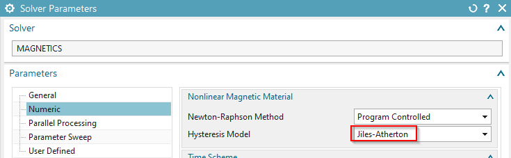
Edit the solver parameters of the solution. Switch to register
’Numeric’. Notice, the ’Hysteresis Model’ is set to ’Jiles-Atherton’.
Thus, the solution will include additional terms for Jiles-Atherton
calculation.
Be aware that these terms are of nonlinear type and will lead to
higher computation time. Thus, also the settings at ’Newton-Raphson
Method’ do have an influence on this computation. In our case all
settings here are at their defaults but other cases may need extra
attention here.
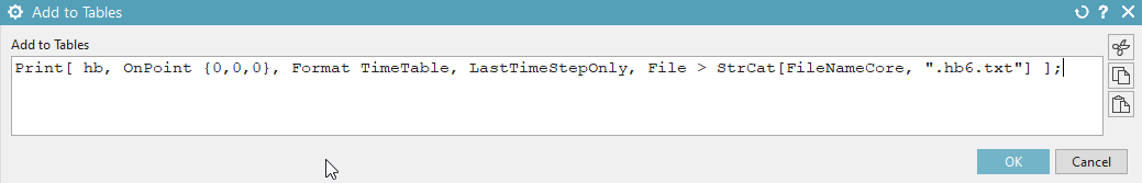
Set the register to ’User Defined’. Notice, in ’PostOperation’,
’Add to Tables’ there is a text entry defined. This leads to writing the
result ’hb’ into a text file with extension ’hb6.txt’ (6 for position
6). The ’hb’ quantity is only for post processing. It contains the x, y,
z components of magnetic field strength (h) and x, y, z components of
magnetic flux density (b). We will later use this output to generate the
hysteresis curve in MS Excel.
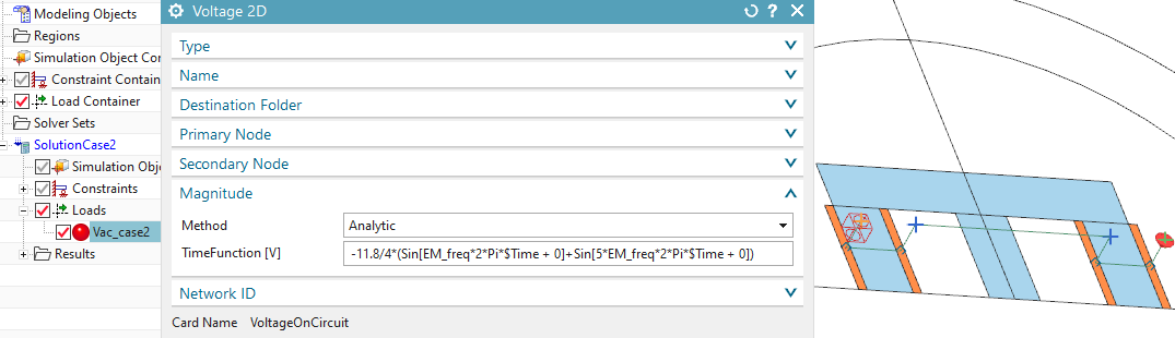
Check the load: Notice, it is a voltage load being applied to the
two coil connectors. The load is defined as ’Analytic’, because this
allows to add the fith harmonic simply by writing the desired formula as
seen in the below picture.
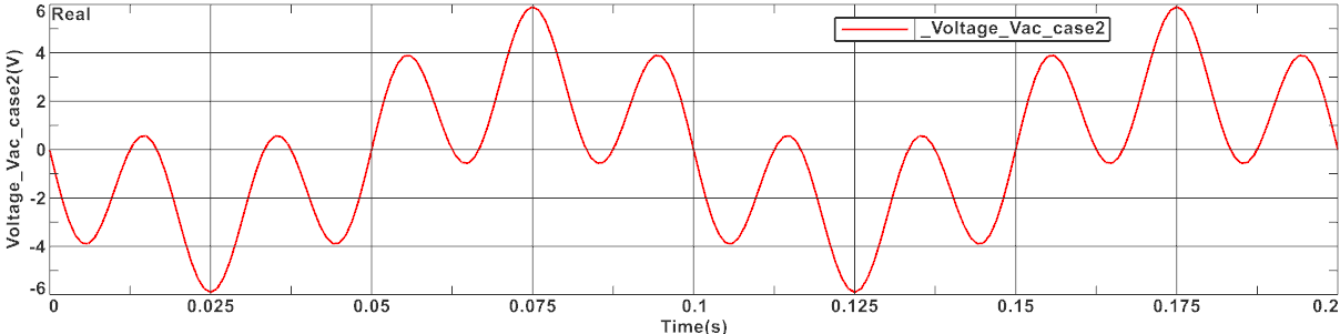
The following picture shows that voltage as a graph.
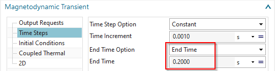
Edit the solution, in ’Time Steps’, set the ’End Time Option’
from ’Number Time Steps’ to ’End Time’. ’End Time’ is then 0.2 sec. Now
the solution will run two times over the sinus period.
Finally, solve the solution. Solve time will be about 3 minutes
for the 200 time steps and nonlinear iterations.
To make a graph b over h and demonstrate the hysteresis effect,
do the following:
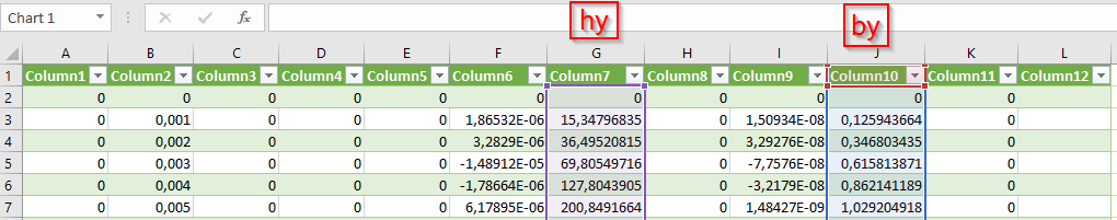
Import the text file ...hb6.txt in Excel (maybe it is cenessary
to replace points by comma first in a text editor).
The file contains in each line the result of one time step. There
are 3 components for h (magnetic field) and 3 for b (magnetic flux
density). Additionally there is the point location and time at the
beginning of the line. We now want to make a graph h over b with the y
components.
In Excel, select the two columns and insert an X Y (Scatter)
graph. It shows the desired magnetic hysteresis curve. The computed
curve (below right) agrees quite well to the reference one (below
left).
The tutorial is complete.
References:
Description of TEAM Problem: 32. "A Test-Case for Validation of
Magnetic Field Analysis with Vector Hysteresis", at the following
Link.
https://www.compumag.org/wp/wp-content/uploads/2018/06/problem32.pdf
Experimental data to the TEAM 32 benchmark is available at the
following link.
http://www.cadema.polito.it/team32
"Using a vector Jiles-Atherton hysteresis model for isotropic
magnetic materials with the FEM, Newton-Raphson method and relaxation
procedure", Guérin C., Jacques K., Sabariego R. V., Dular P., Geuzaine
C. and Gyselinck J.
"Incorporation of a Jiles-Atherton vector hysteresis model in 2D
FE magnetic field computations, Application of the Newton-Raphson
method", Gyselinck J., Dular P., Sadowski N., Leite J., Bastos
J.P.A.
Post-only - Run separate
Post-Processing
Usually, when a solve is performed, the system first does a solve and
then automatically adds a post-processing of the user-requested outputs
(results). The solve may be very time consuming while the
post-processing normally needs much less time. A disadvantage is the
following: If, after such a solve, the user realizes that another result
type may be desired, the whole solve and post-processing work must be
done again. To overcome this there exists the feature ’Post-only’. It
allows to perform post-processing alone. Of course, there must be a
solve that already has run before this. The following steps show such
process.
Open a Sim file and solve a solution.
Edit the solution and change the ’Output Requests’. Activate any
new output and deactivate the existing ones. (Deactivation should be
done because otherwise these old results will be written into the result
file once again even if they are there already.)
Edit the ’Solver Parameter’ of the solution and in register
’General’, activate the bottom ’Solve-only’.
Check that the bottom ’SaveSolution (for later Post-only’ is
activated.
Solve the solution again. Now, only the post-processing step is
done and the newly requested outputs are added into the result
file.
The following known issues exist with this feature:
When the solution uses time steps, the added results will be one
step too early. For instance the result of step 5 will be placed in the
result file as step 4.
Any results of type ’Virtual Force’ (or moment) cannot be used
with the ’Post-only’ feature. The reason is that those results need
separate solves to be done and if this is not active in the main solve
it cannot be post-processed.
This feature is available since NX version 2306. In older versions,
it is available if the Magnetics-installation is done with option ’Use
Typical Installation’: ’N’ (no) and ’Latest Version’.