Tutorial 1 (Beginner)

Three Moving Magnets

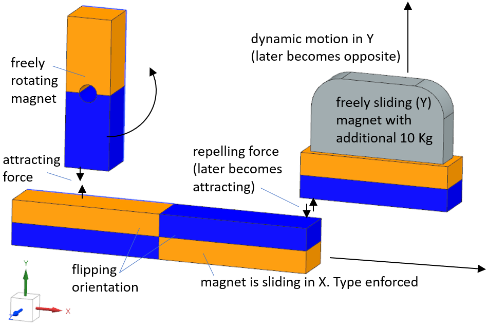
In this tutorial we analyse a system of two slider- and one rotor-magnets. Enforced translation in x is applied to the first slider (bottom in below picture). The other two move freely (dynamic) because of the permanent magnet forces acting on them.

The right slider feels an attracting force and accelerates in positive y direction. An additional weight of 10 Kg makes it’s move slower. Because the bottom magnet flips its orientation, after a while the repelling force becomes attracting and the 10 Kg mass comes back. On the left, there is a rotating magnet that feels attracting force to the below slider. Therefore, it starts rotating in the direction of the slider. When the slider has disappeared, the rotor will continue rotating, only without further acceleration.
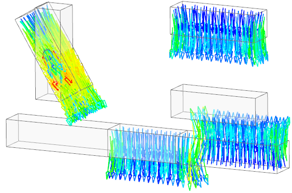
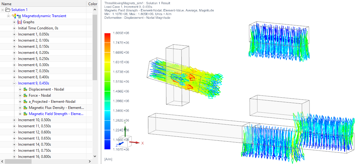
The below picture shows the simulated magnetic field directions at a time short after start.

Main goal of this tutorial is to demonstrate and learn how models with motion can be set up. General Motion is especially useful for such types of 3D motion.

Estimated time: 60 min.

Follow the steps to reproduce it:

Setup Files and Solution

1. Download the model files for this tutorial from the following link:
   https://www.magnetics.de/downloads/Tutorials/6.CouplMotion/6.10ThreeMovingMagnets.zip

2. Extract the zip archive into a folder.

3. Open the part file ’ThreeMovingMagnets.prt’. This is possible in NX 2212 or later versions.

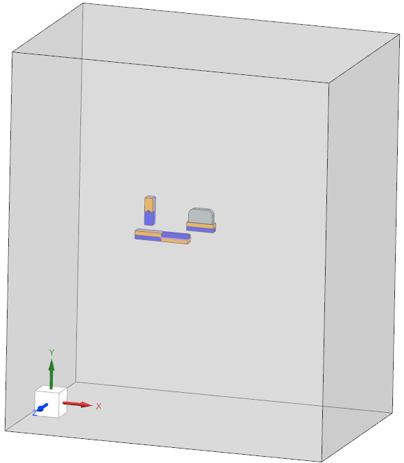
4. Start the Pre/Post application,

5. make sure that all bodies, also the air, are visible,

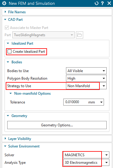
6. create a new Fem and Sim file,

7. switch off ’Create Idealized File’ because it is not necessary,

8. choose the Solver ’MAGNETICS’ and Analysis Type ’3D Electromagnetics’,

9. set the ’Strategy to Use’ to ’Non Manifold’. (in NX 2406 or later this can be simply done in this dialogue, for the prior NX versions, see ’Tutorials EM Basic’, chapter ’Recommended System Settings’, ’Create Non Manifold Polygon Bodies’).
   

10. Click OK.

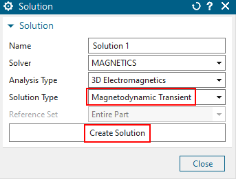
11. If the window ’Solution’ does not appear automatically, click the button ’Solution’,

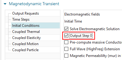
12. in window ’Solution’, set the ’Analysis Type’ to ’Magnetodynamic Transient’ and click ’Create Solution’,

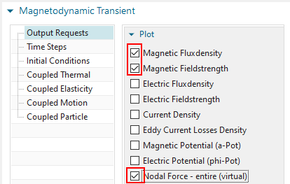
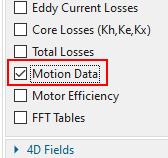
13. in register ’Output Requests’,’Plot’ activate ’Magnetic Fluxdensity’, ’Magnetic Fieldstrength’, ’Nodal Force - entire (virtual)’ and in ’Table’ activate ’Motion Data’. Others can be activated if one is interested,
    

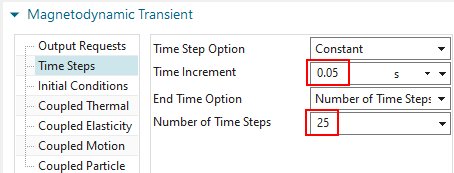
14. in register ’Time Steps’ set the ’Time Increment’ to 0.05 s and the ’Number of Time Steps’ to 25. These settings must be carefully adjusted to find a good time range for the simulation,

15. in register ’Initial Conditions’, activate ’Output Step 0’ to also see the result at the beginning.
    

16. click OK. All other settings are well defined. The file structure is created.

Meshing and Properties of the Permanent Magnets

1. Switch to the Fem File.

2. Blank the polygon body ’Air’ for easier viewing.

3. Notice, that we do not need Mesh-Mating-Conditions, because of the used strategy ’Non Manifold’. Maybe you check in groups ’non-manifold face’. Here all such faces are shown.

4. Optionally, use RMB on the polygon bodies and choose ’Synchronize CAD Properties’ to update the names.

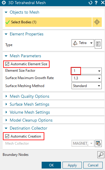
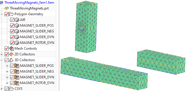
5. Following, use tetra elements and the automatic element size. Mesh all four magnet bodies:
   ’MAGNET_SLIDER_POS’,
   ’MAGNET_SLIDER_NEG’,
   ’MAGNET_SLIDER_DYN’ and
   ’MAGNET_ROTOR_DYN’.
   Use a separate mesh collector for each of them. The below picture shows left the Tetra meshing window and right the resulting meshes and collectors in the navigator.
   

6. Edit the mesh collector and the physical property of MAGNET_SLIDER_POS.
   

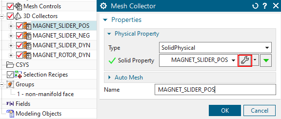
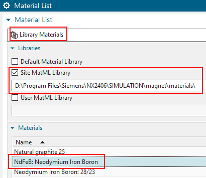
7. For ’Material’, select from the shown library (the shown path may be different) the permanent magnet material ’NdFeB: Neodymium Iron Boron’. You can use any other permanent magnet material but of course the results will differ then.
   

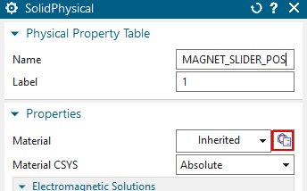
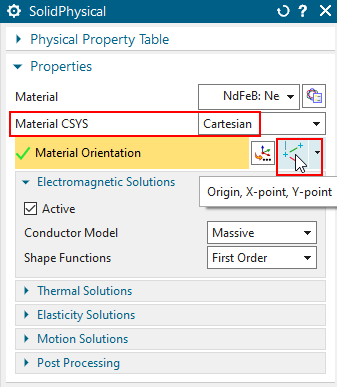
8. Click OK. Back in the window ’SolidPhysical’, we have to correctly orient the magnet direction. Therefore, set the ’Material CSYS’ to ’Cartesian’ and use any of the ’Material Orientation’ methods there (we prefer the method ’Origin, X-Point, Y-Point’) to orient the x axis into the north direction. See following picture for the correct directions of all four magnets. Only x is important, y and z do not play a role.
   

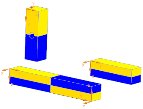
9. In the same way as the first one, edit the remaining three magnets, assign the same material and the corresponding magnet directions.

Defining the Updating Air Mesh

The air between the moving bodies (magnet faces) and the outside (air block faces) must be meshed in a way that it will update at every motion step. Therefore, we use the feature ’Auto Mesh’ that needs to know all bordering faces. This feature is found in the 3D mesh collector window. Proceed as follows:
First, we create an empty mesh collector with the usual properties for air:

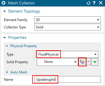
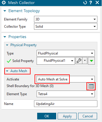
1. Click RMB on ’3D Collectors’ and choose ’New Collector’.

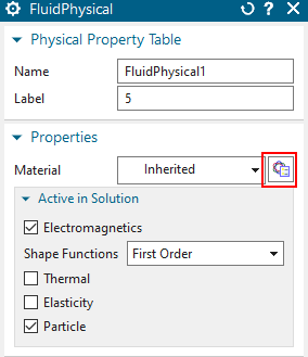
2. Type in a name like ’UpdatingAir’, set the Type to ’FluidPhysical’ and click ’Create Physical’

3. In window ’FluidPhysical’, select ’Material’ and in the ’Material List’, select the shown library and the material ’AIR’.
   

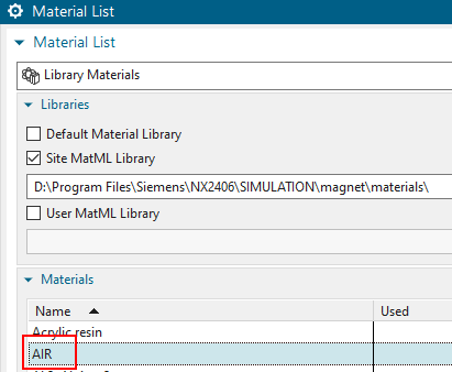
4. Click OK, OK, OK to close the windows. We will later come back here.

Now we create 2D boundary meshes on the magnets and also on the outside faces of the air box. For the magnets, because they already have 3D meshes, we will make coat meshes that simply extract the existing 3D element faces.

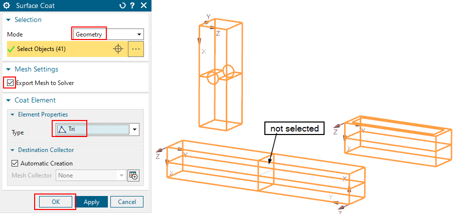
1. From the toolbar, in group ’Mesh’, choose the feature ’Surface Coat’,

2. set the ’Mode’ to ’Geometry’ and select all outside faces of the magnets.

3. Hints: you can drag a window over all, but be careful not to select the two contact faces of the horizontally sliding magnet (picture below). These must not be selected, otherwise the air mesh cannot be created. It is a good idea to check the correct border meshes by manually executing the ’Solid from Shell Mesh’ using these 2D meshes.

4. Set the ’Type’ to ’Tri’ and activate ’Export Mesh to Solver’

5. Click OK to create the coat meshes.

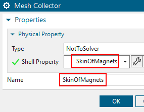
6. For easier finding, rename the newly created 2D Mesh Collector and its physical to ’SkinOfMagnets’. We have to select this later in the ’Auto Mesh’ feature.
   

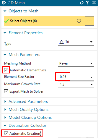
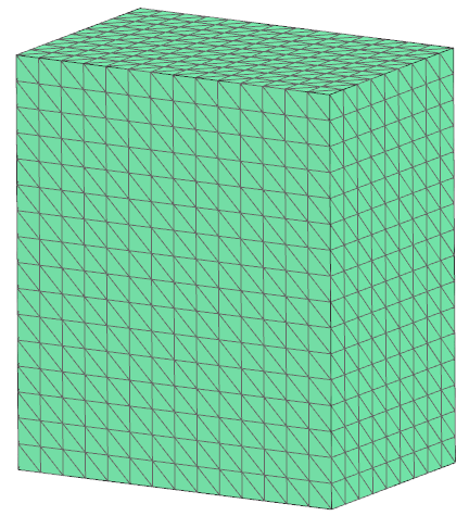
Now, we create usual 2D tri meshes on the air outside border. We use this 2D mesh for the updating air but also for the constraint ’Zero Vectorpotential’ that is necessary here.

1. Unblank the air body and select from the toolbar the ’2D Mesh’ feature,

2. select all six outside faces and set the element size to a quarter of the automatic element size. Click OK to create the mesh.
   

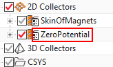
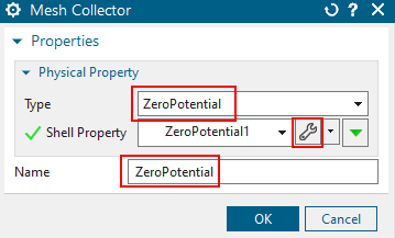
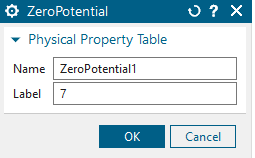
3. Edit the newly created 2D mesh collector, rename it to ’ZeroPotential’ and

4. set the Type to ’ZeroPotential’. Click ’Create Physical’ and OK (no properties are necessary, just the type).
   

Finally, we assign the bordering 2D meshes in the Auto Mesh feature:

1. Edit the mesh collector ’UpdatingAir’, open the box ’Auto Mesh’ and set ’Activate’ to ’Auto Mesh at Solve’

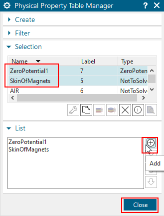
2. At ’Shell Boundary for 3D Mesh’, click on ’Create Shell Boundary for 3D Mesh...’

3. in the following window, select the two physicals ’ZeroPotential1’ and ’SkinOfMagnets’ (maybe you have named them differently) and click ’Add’. So they are added to the list.

4. Click Close and OK to finish.
   

Creation of Motion Joints

The only things we have to do in the Sim file is the creation of motion joints for the three bodies. No currents or any other is necessary because the permanent magnets forces is what we want to analyse here. Only one additional feature we will use is a ’Locally increased Order’ that is useful for higher FEM accuracy on the magnets.
We start with the enforced slider joint for the horizontally moving magnets.

1. Switch to the Sim file.

2. Blank all 2D meshes and also the air polygon body for easier visualization.

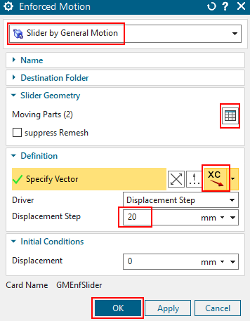
3. Create a ’Simulation Object’ of type ’Enforced Motion’ and set the option to ’Slider by General Motion’.

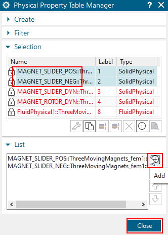
4. In box ’Slider Geometry’, ’Moving Parts’, choose ’Create Moving Parts...’ and in the following window, select the physicals ’MAGNET_SLIDER_POS’ and ’MAGNET_SLIDER_NEG’, click ’Add’ and Close.

5. Set the Vector direction to X and use a ’Displacement Step’ of 20 mm. This means at every time step the joint will move 20 mm in positive x direction.

6. click OK to create the joint and blank it for better visualization.
   

Following, we create the two dynamic joints. One is translating in Y and the other rotating about z direction. Let’s start with the dynamic slider:

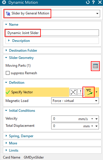
1. Create a ’Simulation Object’ of type ’Dynamic Motion’ and set the option to ’Slider by General Motion’,

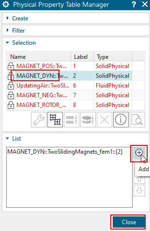
2. At ’Moving Parts’, select the ’MAGNET_DYN’ physical,

3. at Vector direction, select Y,

4. assign as Name ’Dynamic Joint Slider’,

5. click OK to create the joint.
   

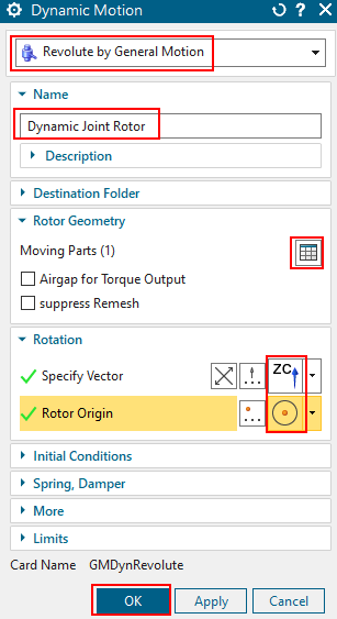
Now the last one, the rotor:

1. Create a ’Simulation Object’ of type ’Dynamic Motion’ and set the option to ’Revolute by General Motion’,

2. At ’Moving Parts’, select the ’MAGNET_ROTOR_DYN’ physical,

3. at Vector direction, select Z,

4. at ’Origin’ select a point in the center of the rotor hole.
   Hint: In MAGNETICS versions prior to 1268, the rotor origin had to be at absolute CSYS origin. As workaround the geometry can be shifted such that the rotor origin becomes that position. Alternatively, the unsigned user interface can be installed to get access to all latest features.

5. assign as Name ’Dynamic Joint Rotor’,

6. click OK to create the joint.
   

Apply Mass and Inertia

Notice that there is no displacement step \(s\) or velocity given for the two dynamic joints because here motion is driven through mass \(m\) and magnetic force \(F\) and time step \(t\) by Newton’s law:

These formulas apply for both translation as well as rotation. Only the properties mass and inertia must be defined. Mass is necessary for translation and inertia is the corresponding property for rotation. Proceed as follows:

1. Switch to the Fem file

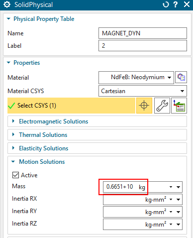
2. Edit the physical properties of ’MAGNET_SLIDER_DYN’,

3. open the box ’Motion Solutions’ and key in the value for mass. Because for the vertical slider we wanted additional 10 Kg mass added, this must be defined here.

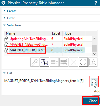
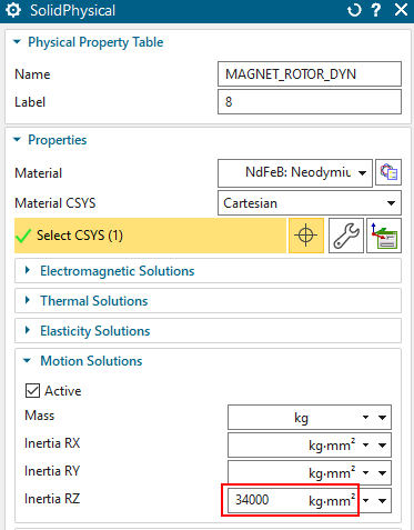
4. Correspondingly for the rotor joint, Edit the physical properties of ’MAGNET_ROTOR_DYN’,

5. At ’Inertia RZ’, key in the shown value.
   Hint: The inertia value of a solid geometry can be calculated by a mass analysis in the CAD system.
   

6. Switch back to the Sim file.

Apply Locally Increased Order

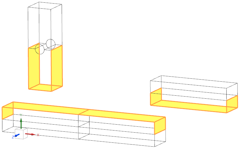
Because the accurate calculation of magnetic forces on permanent magnets requires relatively fine meshes or higher order shape functions we will apply such higher order shape functions. But because these require lots of memory while solving we try to limit their effect to only force responsible faces. In this small model, we could also apply them to larger regions but in large models we should carefully use this. Proceed as follows.

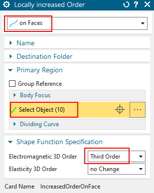
1. Create a ’Simulation Object’ of type ’Locally increased Order’,

2. set the option to ’on Faces’ and select the faces as in the picture below.

3. At ’Electromagnetic 3D Order’, set the option to ’Third Order’,

4. click OK to create the feature.
   

Run the Solve with General Motion

If General Motion (GM) is running, the NX mesher is called once every time step for the update of the air mesh. During the process NX shows nicely the meshes and how they are moving. But the user cannot modify anything. The NX window is blocked and that’s why we recommend resizing it some smaller. This allows doing some other work on the computer. Further, if the information window pops up over the graphics area, we cannot see any more the moving. Thus, it it a good idea to prior move the information window outside the graphics area.

1. Save the files.

2. Resize the NX window to a smaller size (maybe the half or quarter of the whole screen),

3. open the information window by using Menu, Information, Object, select anything, OK.

4. drag the information window to a place somewhere outside the NX graphics area.

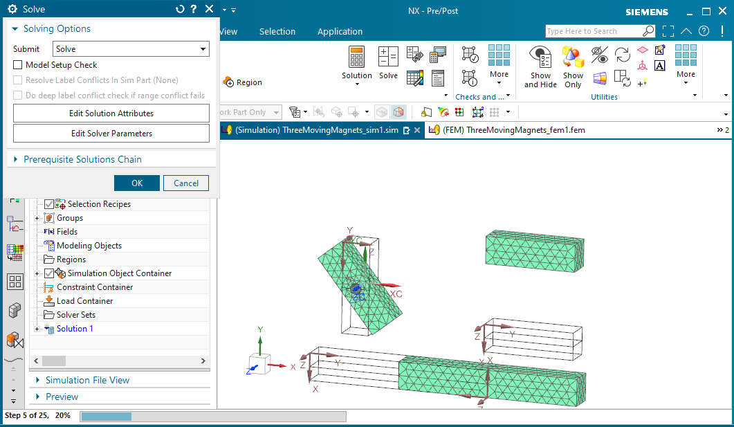
5. Click ’Solve’ and OK. The solve begins.

6. observe in the NX graphics window the motion and the progress line at the bottom left. The solve will take about 5 or 10 minutes on a usual computer.
   

7. Sometimes it is desired to interrupt a General Motion run prior to the final time step. For that purpose a bat file is created in the work folder with file extension ".Click2InterruptAtNextStep.bat". This file can be executed (double click) during solve and as soon as the current time step is finished the process is stopped. All results until that time will be written and can be post processed.
   Hint: Alternatively, the user can create a file (text file or any other) with the core name of the simulation (e.g. like all the other files in the folder) and with extension ".break". This will have the same effect as the above "Click2InterruptAtNextStep.bat".
   Alternatively, a brutal way to stop the solve is to kill the ’ugraf.exe’ process and also the solver ’MagneticsSolveR.exe’ by the task manager.

Post Process Motion Results

As soon as the General Motion process has finished the results can be opened and post processed as usual.

1. Double click the node "Results". For each time step there is one set of results created.

2. the following picture shows some of the tabular results (velocity and total displacement of the dynamic joints)
   

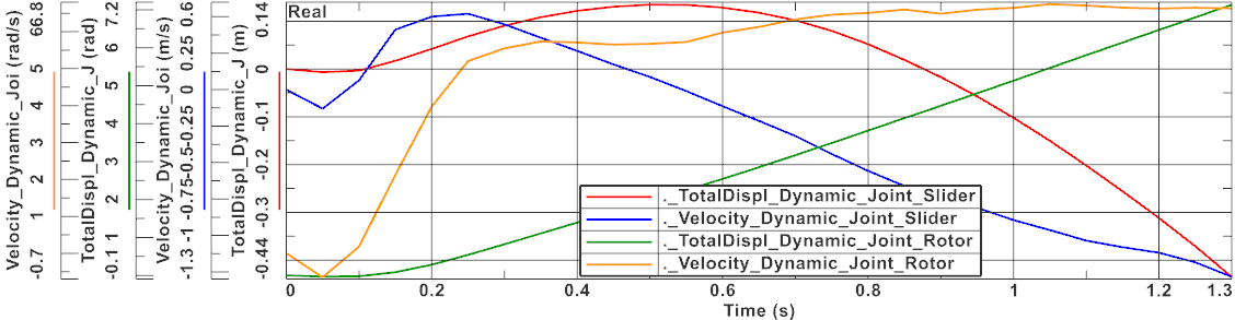
3. and the resulting magnetic fieldstrenght in the middle of the time period. The un-deformed geometry is also displayed here.
   

Some useful Options for General Motion

In Edit solution, register ’Coupled Motion’, there are two features that we want to explain:

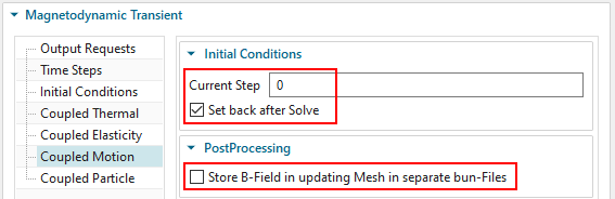
• ’Set back after Solve’. The option is active by default. If deactivated, the motion can be continued from the prior run. E.g. the meshes stay in the last position and all information about velocity of the joints is kept as initial condition. Thus, only the number of time steps must be increased and the motion will continue from that when solving.

• ’Store B-field in updating Mesh in separate bun-Files’. This option is off by default. Unfortunately, the results on the updating mesh cannot be stored together with the usual mesh. Thus, we cannot see, e.g. magnetic fluxdensity in others than the initial time step. To overcome this problem, one can activate this button. The resulting files, one for each step, can then be imported into the post processor and analysed. This feature is available in MAGNETICS versions 1268 or later.

The tutorial is complete.