This chapter again deals with heating of conductors. Additionally to
the chapter before, thermal solutions are now performed by the solver(s)
Simcenter Thermal/Flow or ESC (Electronic Systems Cooling). Main
advantages of these processes come from the flow cooling effect that is
now captured precisely with CFD simulation instead of using simple fixed
convection coefficients as we did before.
The Magnetics solver again computes the electromagnetic fields with all
corresponding skin- and proximity effects and eddy-current-losses. If
the electric current is only DC, the Magnetics solution would even not
be necessary, because this kind of pure electric load can be modeled
completely in Simcenter Thermal/Flow(ESC) by the feature ’Joule
Heating’. As soon as AC or transient currents play a role, this can not
be modeled by ’Joule Heating’ any more, because of induction effects
that must be simulated by dynamic electro-magnetic solvers.
Focus in the tutorials will be on the transfer of such losses from
Magnetics to Thermal. But also material properties being temperature
dependent play a role. The reader should already be familiar with the
solver Thermal/Flow or ESC.
Conductor
Heating with Flow Cooling
One Way Coupling
In this tutorial we start with a quite simple process: First
computing the eddy current loss by the Magnetics solver. The result is a
single integral value in unit watt (W). Then, using the
Thermal/Flow(ESC) solver, we assign that loss value as a load and
compute temperatures.
The result of such a simulation is of acceptable quality, it includes
the dynamic electromagnetic effects, but it does not capture the spatial
distribution of losses. Thus, if more accuracy is required, we can use a
loss field instead of the integral value. Below, we show both ways,
marked as ’Alternative 1’ and ’Alternative 2’.
Secondly, not taken into account with such simulations are temperature
changes that lead to changes of material properties (mainly the electric
conductivity). Thus, this is a simplified process and this limitation is
carried out in following tutorials.
Hint: The model is already build and ready to solve. In this tutorial we
go through the existing features to check and explain them.
Follow the steps:
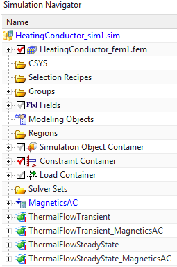
Start Simcenter and open the Sim file
’HeatingConductor_sim1.sim’.
Check solution ’MagneticsAC’
Edit the solution. This is a Magnetics solution of type
’Magnetodynamic Frequency’. So, it is possible to compute AC with eddy
current losses here.
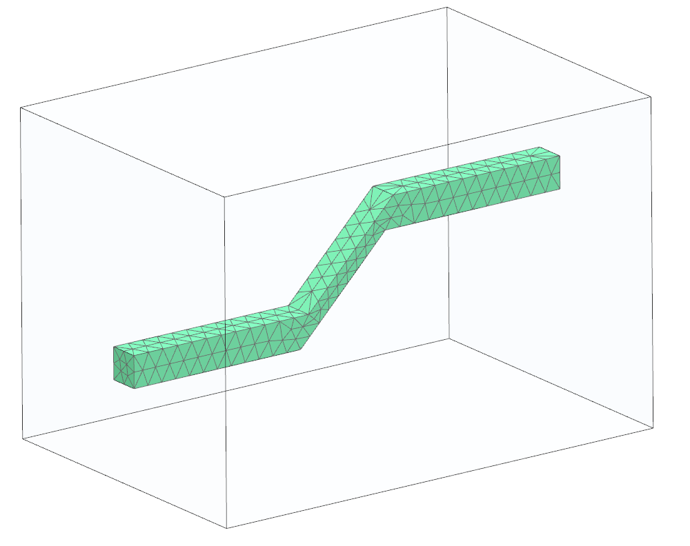
Hint: This solution and model is quite similar to the AC simulation of
the previous chapter. Only, the air mesh uses boundary layer elements
for more accurate wall conditions.
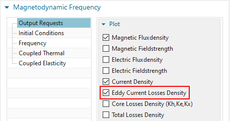
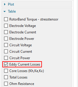
Check the settings in register ’Output Requests’:
The option ’Eddy Current Losses’ in box ’Table’ is the important
output because it computes the integral value of losses. These losses
are assigned as load in the Thermal/Flow or ESC solution.
The option ’Eddy Current Losses Density’ in box ’Plot’ is also
active. This output is necessary to create a loss field with spatial
distribution. Such a loss field can be used alternatively to the
above.
Hint: Instead of ’Eddy Current Losses’, we can also use ’Total Losses’.
Such total losses contain eddy current losses plus core losses. To
activate core losses, the material property Kh (Ke, Kx) must be set
larger than zero. Kh models hysteresis losses resulting from changing
magnetic fields.
Check the solution ’ThermalFlowSteadyState’.
This is a coupled Thermal/Flow solution. So, it computes
temperatures, fluid velocities and pressures.
There is a inlet flow velocity of 5 m/s defined in z direction
what leads to a cooling effect.
In the ’Results Options’, ’3D Flow’, there are the convection
coefficients requested.
the Fem file contains both Magnetics and Thermal/Flow properties.
The Magnetics properties can be seen, when the solver is set to
MAGNETICS (Fem part, Edit) and the Thermal/Flow properties can be seen,
when it is set to that solver.
We will solve this steady state solution but notice, there is
also a transient solution ’ThermalFlowTransient’ that can also be solved
to simulate transient heating.
Solve the solution ’MagneticsAC’.
After the solve has finished, check the requested loss on the
conductor in the corresponding text file ’*.EddyCurrentLosses.txt’. It
is approximately 20 W.
If there are any 2D conductors (electric interface resistances or
conducting sheets) in the model, the text file would also contain the
losses values for these.
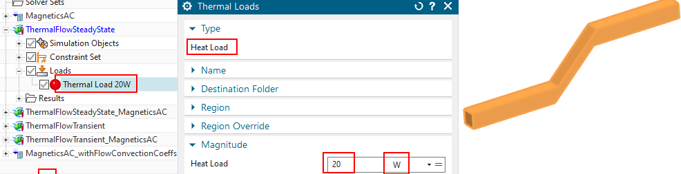
Transfer losses, use integral value (Alternative
1)
Activate solution ’ThermalFlowSteadyState’ and check the existing
load ’Thermal Load 20 W’. This is a ’Thermal Load’ of type ’Heat Load’,
expecting the unit W and it is assigned to the solids. Therefore, this
load type is convenient to transfer the integral loss value on solids
from Magnetics.
If there are any 2D conductors (electric interface resistances or
conducting sheets) in the model (not in the tutorial model, see picture
below for an example), these would need additional loads assigned to
those faces with their corresponding loss values.
Transfer losses, use spatial field (Alternative
2).
While the above method (integral loss value) does not capture any
spatial distribution of losses, there does exist an alternative way that
overcomes this issue: The losses density can be stored as a spatial
field in Simcenter. Then, in Thermal/Flow environment, such loss field
is referenced in the heating load. Proceed as follows for this
alternative:
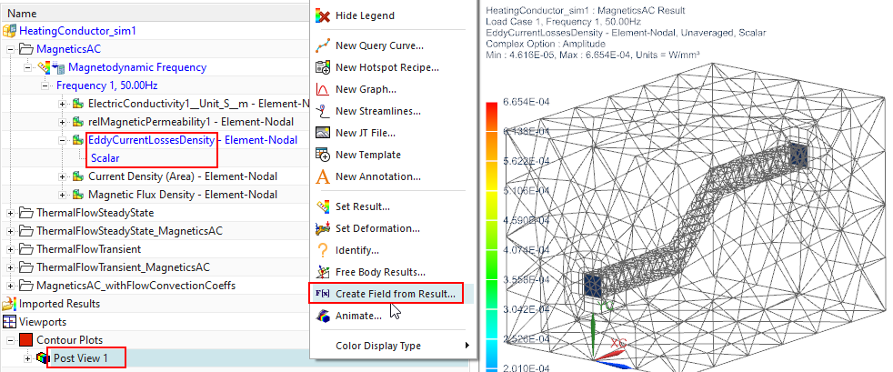
Display the magnetic losses result on solids (either
’EddyCurrentLossesDensity’ or ’TotalLossesDensity’) in a post view (see
picture below).
If there are any 2D electric interface resistances or conducting
sheets in the model:
There will be an extra result ’EddyCurrentLossesDensityArea’,
unit \(W/mm^2\).
That result must be stored in a separate field because of the
different unit.
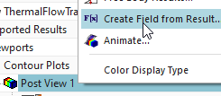
Right mouse button on the ’Post View’, choose ’Create Field from
Result’.
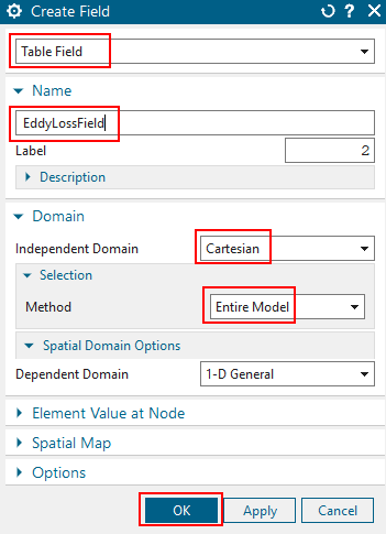
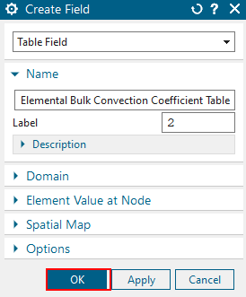
The dialogue ’Create Field’ appears. See picture below left
side.
Key in for name ’EddyLossField’ (or similar). All defaults can be
accepted.
Hint: Accept the default ’Independent Domain’ of ’Cartesian’.
This setting allows using different meshes for the electromagnetic and
the thermal solutions, because interpolation is used.
Hint: Accept the default ’Selection Method’ ’Entire Model’.
Because the air does not have any loss results, it will not be written
into the field.
Click OK and the field is created.
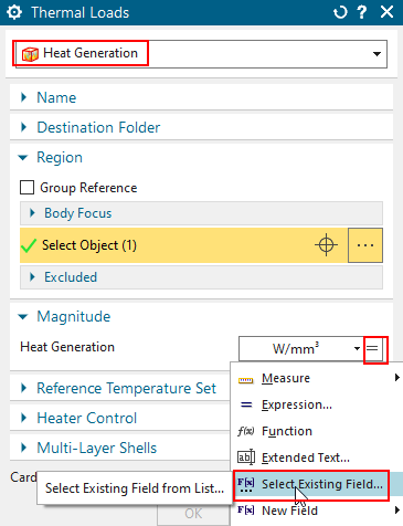
Activate solution ’ThermalFlowSteadyState’. (Remove the existing
load ’Thermal Load 20W if working on the tutorial model)
Create a new ’Thermal Load’. See picture above right side. Set
the type to ’Heat Generation’. This type expects the unit \(W/mm^3\) that corresponds to the Magnetics
losses density on solids.
Select all solid conductor bodies.
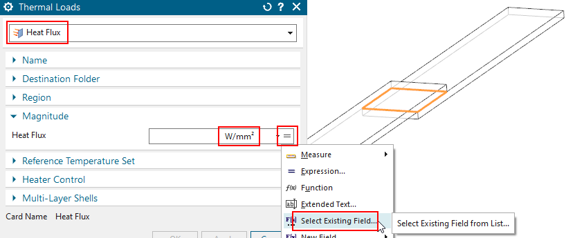
Instead of keying in a single loss value, choose ’Select Existing
Field’ and in the following window select the previously created field
(EddyLossField). Click OK, OK.
In case there are any 2D interface resistances or conducting
sheets in the model:
This is not in the tutorial model, see picture below for an
example.
There should already be a separate field previously created for
their losses.
Create an additional ’Thermal Load’ but now use the type ’Heat
Flux’ because this expects the unit \(W/mm^2\) that corresponds to the 2D
losses.
Select the faces of such 2D interface resistances or conducting
sheets.
Choose ’Select Existing Field’ and select the previously created
field.
Solve the solution ’ThermalFlowSteadyState’.
After the solve has finished, feel free doing any post
processing.
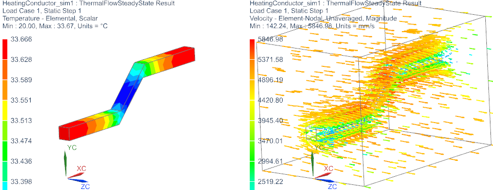
Following picture left shows the computed solid temperatures with
a maximum of \(33.6^0 C\) and right the
fluid velocity.
The advantage of this type of solution becomes clear: The flow,
coming from the side, leads to a conductor cooling that can not be
easily modeled by fixed convection effects. Thus, a pure Magnetics solve
cannot capture this. One possibility to overcome this is shown in the
following chapter: ’One point five Way Coupling via Convection
Coefficients’.
The tutorial is finished.
One point
five Way Coupling via Convection Coefficients
The Simcenter Thermal/Flow(ESC) solver has the powerful capability of
finding accurate local heat transfer convection coefficients (HTC). At
each element face of a fluid-solid interface, the CFD method calculates
such an coefficient, taking into account the local fluid velocity,
turbulence characteristic and fluid temperature. Such coefficients can
be computed once by the Thermal/Flow(ESC) solver and then reused by NX
Magnetics’ internal thermal solver. This allows doing different kinds of
EM/Thermal simulations all in NX Magnetics, without the need for the
Thermal/Flow solver any more. Following, we show how this is done.
We begin from the model of the previous chapter. Open the Sim
file ’HeatingConductor_sim1.sim’. This model contains Magnetics and
Thermal/Flow solutions from the previous chapter.
Activate the solution ’ThermalFlowSteadyState’.
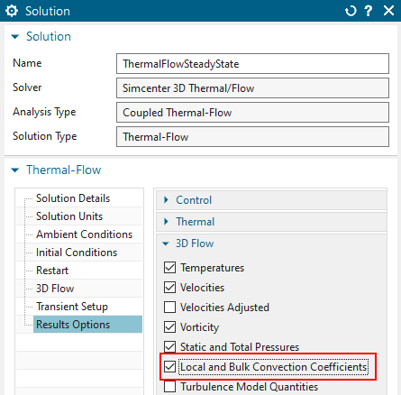
Activate the output of the thermal convection coefficients: Edit
the solution and in register ’Results Options’ in Box ’3D Flow’,
activate ’Local and Bulk Convection Coefficients’ (see picture below,
left). In the tutorial model, the button is already activated.
Hint: The bulk convection coefficients are related to the ambient
temperature (usually \(20^0 C\)). And
the local coefficients are related to the local fluid temperature near
the wall. So, we will use the bulk type because we know the ambient
temperature only.
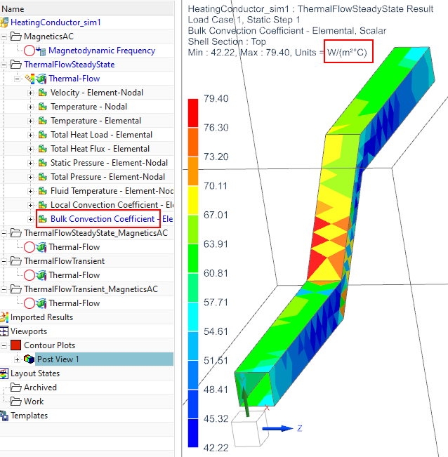
Solve the model and display the result ’Bulk Convection
Coefficient’.
The convection coefficients, as seen in picture above, right are
shown in SI units \(W/(m^2 C\)). In
’Edit Post View’, ’Result’ the unit can be changed. In this example,
they vary between 42 and 79.
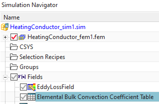
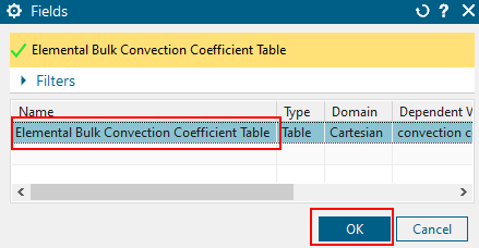
Create a field from this result: Edit the Post View and select
’Create Field from Result’. In the following dialogue ’Create Field’,
accept all defaults and click ’OK’. The Simulation Navigator shows the
newly created field (picture below).
Now, the field with accurate convection coefficients can be used in
NX Magnetics for coupled thermal solutions. To do so, proceed as
follows:
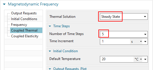
Edit the solution ’MagneticsAC_withFlowConvectionCoeffs’ and in
register ’Coupled Thermal’, set the ’Thermal Solution’ to ’Steady State’
(or transient if desired). Set the ’Number of Time Steps’ to 5 to allow
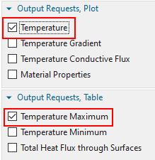
material property updates. Activate the ’Temperature’ plot output
request and the ’Temperature Maximum’ table output request. These
parameters are already set.
Delete the constraint ’Thermal Convection with Coefficients
Field’. We will create this one in the next steps.
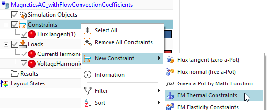
Create a constraint of type ’EM Thermal Constraints’. Set the
type to ’Convection and Radiation to Environment’.
Blank all meshes and the Air body and drag a window over all
faces of the conductor. Deselect the two electrode faces.
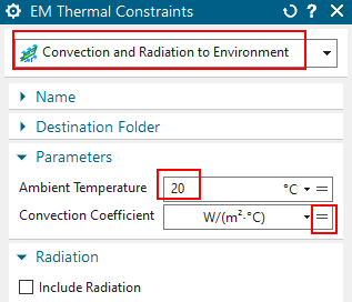
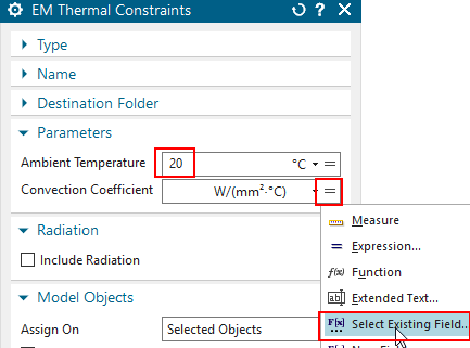
Key in the same ’Ambient Temperature’, that has been used in the
flow solution (\(20^0 C\)), that was
used to find the convection coefficients. This step is important because
the convection coefficients are only valid for one ambient
temperature.
At ’Convection Coefficient’, click on the \(=\) symbol and select ’Select Existing
Field’. In the following window, select the newly created field with the
convection coefficients, Click OK, OK to finish the process.
Hint: The units are automatically set to those of the field. No need to
change them here.
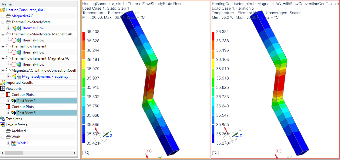
Solve the solution and display the temperature result. Compare
the result with that of the Thermal/Flow solution
’ThermalFlowSteadyState’ (that gave us the convection coefficients).
Both solutions should show results in good agreement. The picture below
shows left the Thermal/Flow and right the NX Magnetics result. The
agreement of the two results becomes even better, if the Thermal/Flow
used the eddy current losses spatial field (above called as Alternative
2).
Advantages of this kind of 1.5 way coupling arises as soon as
following simulations are required. For example, we want to do transient
heating of the conductor. As long as the outside flow stays the same,
convection characteristic (and thus the coefficients) will be influenced
only very little from changes in the electromagnetic solution.
Therefore, we can reuse the field with the convection coefficients and
don’t need updates to the costly Thermal/Flow solution.
The tutorial is complete.
Two Way
Coupling via Plugin Solver
This example demonstrates heating of conductors with use of Simcenter
Thermal/Flow (or ESC) solvers and Magnetics in deep integration.
Therefore Thermal/Flow computes temperature fields and flow velocity
using eddy current losses as input. Magnetics updates material
properties with new temperatures and computes for new electromagnetic
fields and eddy current losses. The two solvers run alternating,
controlled by Thermal/Flow. So Thermal/Flow acts as the master and calls
Magnetics after a defined number of iterations.
The model is already build and ready to solve. In this tutorial we go
through the existing features to check and explain them. Follow the
steps.
Start NX / Simcenter in version 12 or later.
Activate the Plugin (necessary only once)
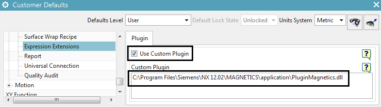
Open the Customer Defaults (File\(\rightarrow\)Utilities\(\rightarrow\)Customer Defaults)
Navigate to Simulation\(\rightarrow\)Pre/Post\(\rightarrow\)Expression Extension.
Activate ’Use Custom Plugin’ and key in the full path and file
name corresponding to your Magnetics installation as shown in the
picture below.
Click OK and restart Simcenter to make the modification
active.
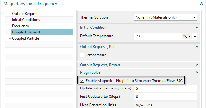
Edit the solution. Click on register ’Coupled Thermal’
Notice in box ’Plugin Solver’ the ’Enable Magnetics-Plugin ...’
button is activated. Through this setting Magnetics will write eddy
current losses into a file (.P.pos) that will be used by Thermal/Flow.
Also Magnetics will write a file (.Plugin.ini) that is used to control
the iterative process.
Notice in the same box the setting ’Update Solve’ is set to 5.
This means Magnetics will be triggered every fifth time step from
Thermal/Flow.
Close the window.
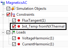
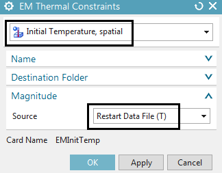
Check the constraint named as ’Init_Temp fromNXThermal’. This is
a ’EM Thermal Constraint’ of type ’Initial Temperature, spatial’. It
allows defining initial temperatures as a spatial field. Through this
feature the Thermal/Flow solver will transfer the resulting temperature
distribution into Magnetics. Magnetics will use these temperatures to
update the materials with those temperatures and perform a new solve.
This feature works similar as a reference-field, but it is more direct
between the two solvers.
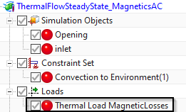
Activate the solution and check settings as desired. There is
nothing special in this solution, all settings are defaults.
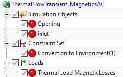
While this is a steady-state solution, there is also a transient
solution named ’ThermalFlowTransient_MagneticsAC’ available (picture
below right) that can be used to solve for the transient heating with
Magnetics update.
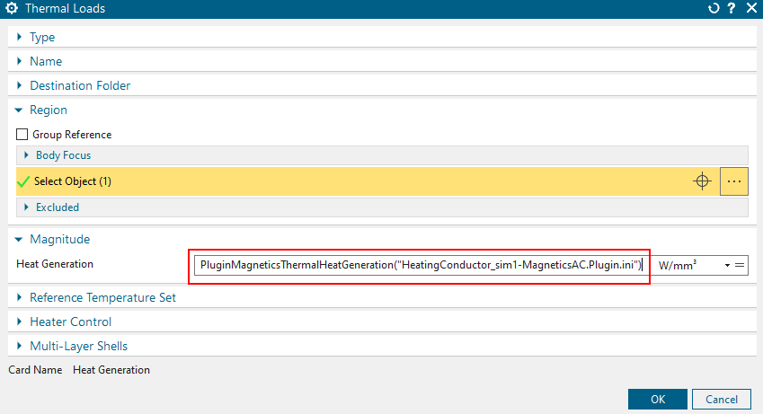
Check the load named ’Thermal Load MagneticLosses’ (see picture
below). This is a load of type ’Heat Generation’. It expects the load in
unit \(W/mm^3\).
Notice, instead of a fixed load value, there is a plugin function
assigned to that load. That plugin function is named
’PluginMagneticsThermalHeatGeneration’ and it takes as argument the name
of a control file pointing to the Magnetics solution:
’HeatingConductor_sim1-MagneticsAC.Plugin.ini’. Hint: This ini file is
automatically created from the Magnetics solve.
In this load, there must be all conductor bodies selected (only
one in our case). Thus, the eddy current losses are applied here
only.
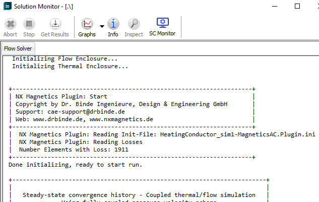
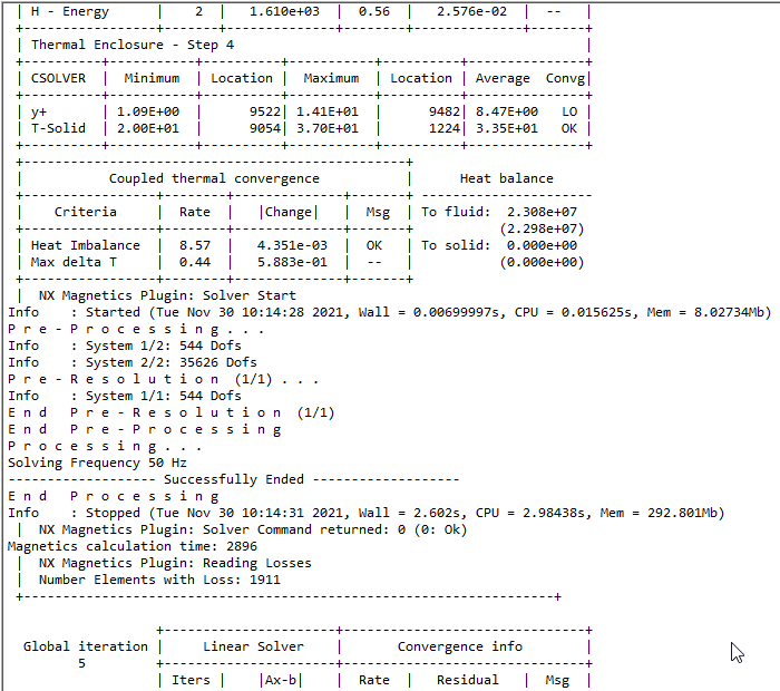
The solution monitor shows the start of the Magnetics
plugin.
Then, every 5th iteration, Magnetics is called to update the
solution.
After the solve has finished, feel free doing any post
processing.
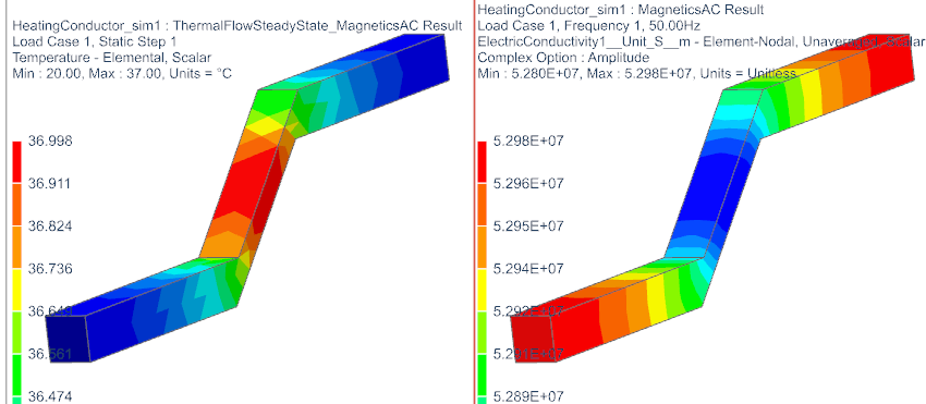
Following picture (left) shows the solid temperatures with a
maximum of 37 \(^0 C\).
The picture right shows the resulting electric conductivity in
unit S/m. This is computed from the magnetic solution and it is
displayed because the output request ’Material Properties’ is activated.
Verify from the two pictures: If temperature (left) is higher, electric
conductivity (right) is smaller.
The tutorial is finished.
Two Way
Coupling via Manual Process
This chapter demonstrates another alternative for the heating of
conductors with use of Simcenter Thermal/Flow (or ESC) solvers and
Magnetics. The coupling is carried out in a manual way while the
previous chapter showed a plugin feature to perform this automatized.
The manual process runs as follows:
The Magnetics solve is first performed. The thermal initial
condition is default, e.g. all materials have \(20^0 C\). The losses result is stored in a
reference field (This approach is demonstrated in the previous chapter:
7. Transfer Losses, use Field).
Next the Thermal/Flow or ESC solver runs. It uses the previously
defined reference field with losses as load (as shown before). The
resulting temperatures on the conductor are stored in another reference
field. This second field must be a ’Elemental Temperature Reference
Field’ and it is created as follows.
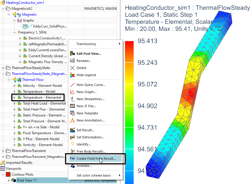
In the post processor display the result type ’Temperature
Elemental’. See picture below left.
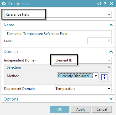
RMB on the ’Post View’ choose ’Create Field from Result’. The
dialogue ’Create Field’ appears. Set the option to ’Reference Field’ and
click ’OK’. See picture below right.
Now, to perform an update, the Magnetics solver gets a initial
thermal constraint that uses the (second) reference field containing the
temperature field. Using this initial condition the Magnetics solver is
started and after finishing the updated losses are automatically stored
in the existing (first) reference field.
From now on the user can alternately start the two solvers. The
maximum temperature should increase slightly and with each iteration
this increase will reduce, ending in a converged situation.
Therefore Thermal/Flow computes temperatures in the conductor and
flow velocity using eddy current losses as heating load. Magnetics reads
the temperature field on the conductor and updates material properties
for those temperatures. Following Magnetics computes new electromagnetic
fields and eddy current losses. The two solvers run alternating,
controlled by the user.
The tutorial is finished.