Estimated time: 1 h
Follow the steps
This chapter shows different ways of electromagnetic heating problems
and corresponding simulations. They are all solved using the Magnetics
solver and the internally, tightly coupled thermal solver. This thermal
solver can handle thermal conduction, convection with fixed
coefficients, radiation to environment and some more basic boundary
conditions. If additional thermal effects must be captured, there exists
the possibility to couple to different solvers like Simcenter
Thermal/Flow or ESC, what is shown in later chapters of this
guide.
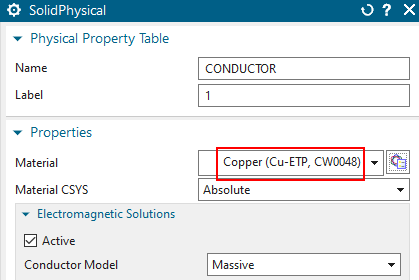
For the conductor body of all following simulations, we use the material
’Copper (Cu-ETP, CW0048)’ with properties from ’Deutsches
Kupferinstitut, www.kupferinstitut.de’.
Important for understanding the differences between the tutorials is to make clear, how the different solution types are defined. The simulation is divided into two domains. The electromagnetic domain and the thermal domain. Each of them can be defined as transient or steady state. A transient defined thermal domain means a temperature which varies over time. The steady state simulation gives the value of the converged transient temperature. Transfered to the electromagetic domain the load (current or voltage) is defined either transient or steady state. Transient means a changing load over time, steady state means the value of the settled transient load. The current can either be DC or AC.
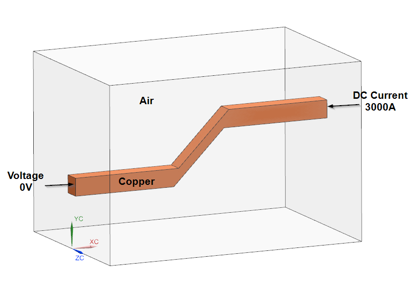
A conductor is heating up due to DC current of 1500 A. The solution
will use a constant current, analyse for the transient electromagnetic
field and temperature distribution. The results are compared against
simple analytic analysis methods. Some following examples build on top
of this one. They analyse for the steady state temperature of the
conductor, and for AC conditions.
Estimated time: 1 h
Follow the steps
Download the model files for this tutorial from the following
link:
https://www.magnetics.de/downloads/Tutorials/7.CouplThermal/7.1HeatingConductor.zip
Open the CAD part file ’HeatingConductor.prt’.
Start Simcenter Pre/Post, load the CAD part and create a new FEM and Simulation using Solver ’Magnetics’ and ’Analysis Type’ ’3D Electromagnetics’. Switch off the idealized part. For the creation of the solution use the following settings:
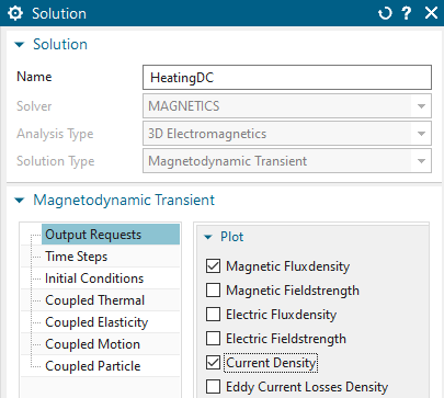
Name the solution ’HeatingDC’,
Use the Solution Type ’Magnetodynamic Transient’,
Hint: This solution type will find the dynamic electromagnetic fields in
the conductor and in the air. A simplification would be to use the ’DC
Conduction Steady State’ solution that would solve only in the
conductor.
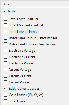
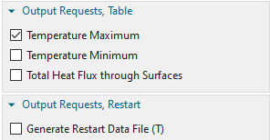
In register ’Output Requests’:
In Plot: Activate ’Current Density’,
In Table: ’Eddy Current Losses’.
Hint: Instead of the Eddy Current Losses, one can also use the ’Total
Losses’. The total losses are eddy + core losses and in this example, we
will not activate core losses.
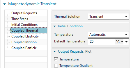
In register ’Coupled Thermal’: Set the ’Thermal Solution’ to
’Transient’ and accept the default initial temperature of \(20^0 C\) to assign this temperature as
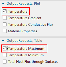
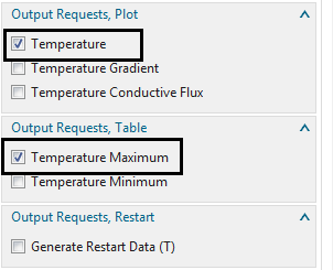
default condition to all temperature conducting parts. Check that the
output request ’Temperature’ is on and activate ’Temperature
Maximum’.
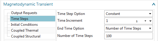
In register ’Time Steps’: Our solution time will be done in 100
steps, each with an increment of 1 seconds.
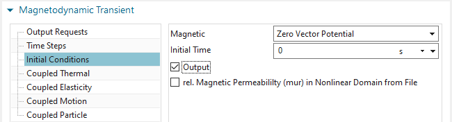
In register ’Initial Conditions’: Activate ’Output’ to get the
initial time step result written into the result files.
Click OK.
Switch to the Fem file
If the ’Early Access Feature for Electro Magnetics’ is not ’On’ (see chapter ’Recommended Settings’), Mesh-Mating-Conditions (MMC) over all geometry now have to be created. If the feature is ’On’, MMCs are not necessary. In that case it only may be checked that the group ’non-manifold face’ shows the correct adjacent faces.
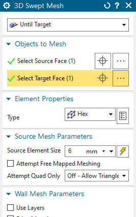
Mesh the conductor using hex elements (tets are also possible).
Choose an appropriate element size (i.e. 6 mm).
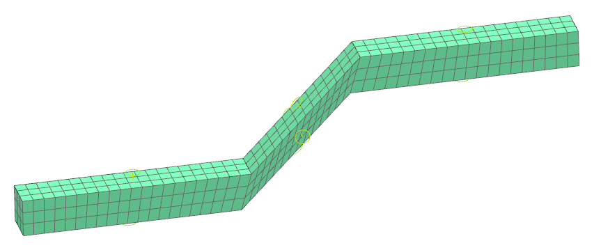
Mesh the air volume with tets.
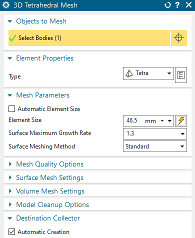
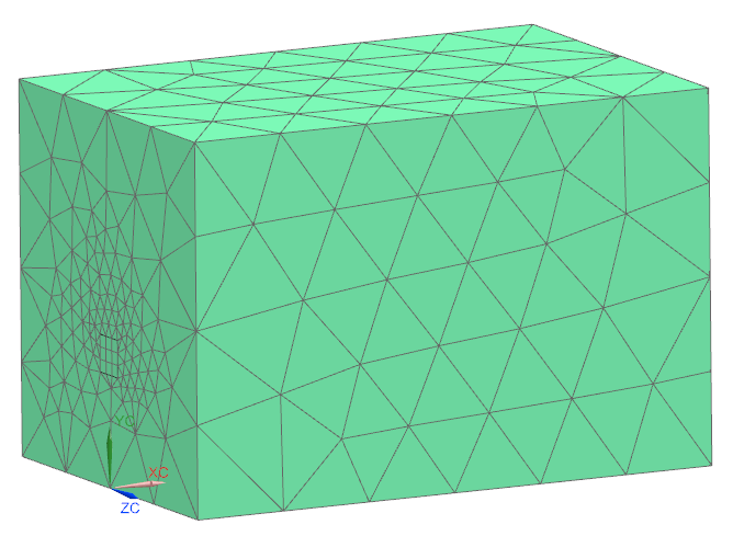
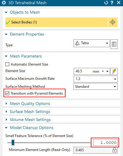
If MMCs are used, the creation of pyramids for perfect transition
is possible as seen in the below picture.

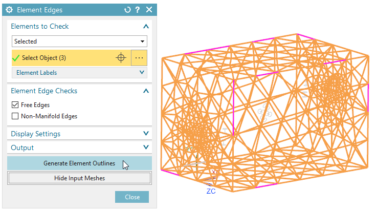
Maybe you do a check ’Element Edges’ and verify there are no free
edges inside the whole region.
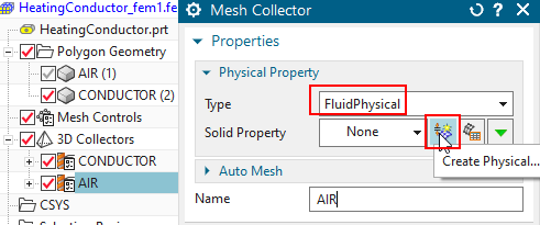
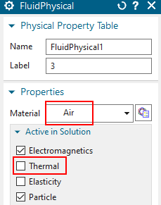
For the ’Air’ mesh-collector, use a physical of type ‘FluidPhysical’ and choose the material ’Air’ from the Magnetics material library.
At ’Active in Solution’, check that ’Thermal’ is deactivated
(default). The conductor will not be solved thermally.
Hint: This is necessary, because we later will apply thermal convection
on the conductor outside walls. Thus, these convection coefficients will
describe the thermal loss of the conductor. If the air would be
additionally active, we would additionally simulate thermal loss from
the thermal conduction between the copper and air.
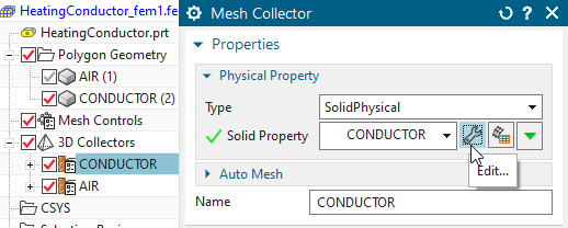
Assign material the ’Copper (Cu-ETP CW0048)’ from the magnetic
library to the conductor. The important material properties are
explained in the following (To check them, use the ’Inspect’ button on
the material).
In register ’Thermal’, all properties for the thermal simulation are
defined. These are:
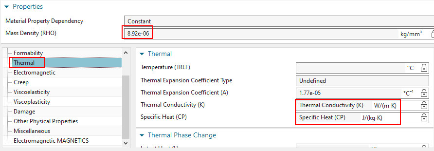
Material ’Mass Density (RHO)’ together with
’Specific Heat (CP)’. These both are necessary to model transient thermal effects.
The ’Thermal Conductivity (K)’ is needed for thermal conduction.
In register ’Electromagnetic MAGNETICS’ the properties for the
magnetic problem are defined as follows.
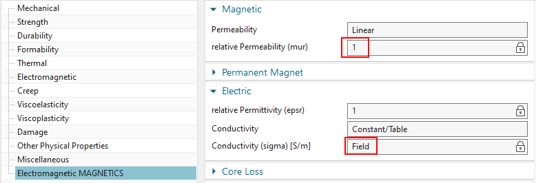
In box ’Magnetic’: The ’relative Permeability (mur)’,
In box ’Permanent Magnet’: The ‘Remanent Magnetic Fieldstrength X’ in case of permanent magnets and
in box ’Electric’: The electric ‘Conductivity (sigma) [S/m]’.
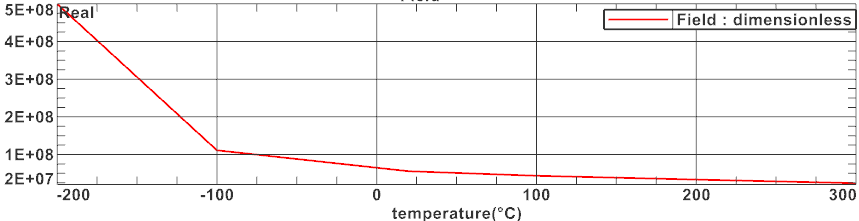
Several properties are defined temperature dependent, as seen in
the below picture for electric conductivity [S/m]. Tables are recognized
by a text-name in the corresponding field instead of a numeric
value.
Switch to the Sim file, blank all meshes.
Create loads and constraints for the usual electromagnetic part of the problem as follows.
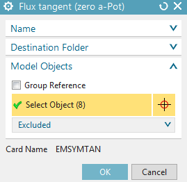
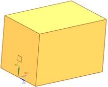
Create a constraint of type ’Flux tangent (zero a-Pot)’ to all 8
outside faces of the air-volume. Assign this condition also to the two
electrode faces of the conductor.
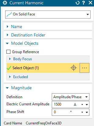
Assign a load ’Voltage’ of type ’On Solid Face’ to one of the
electrode faces of the conductor. Assign a value of ’0 V’.
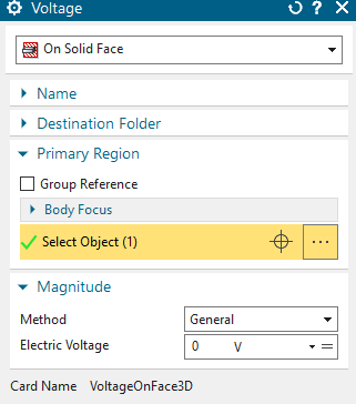
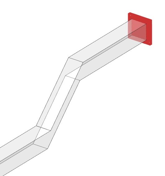
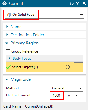
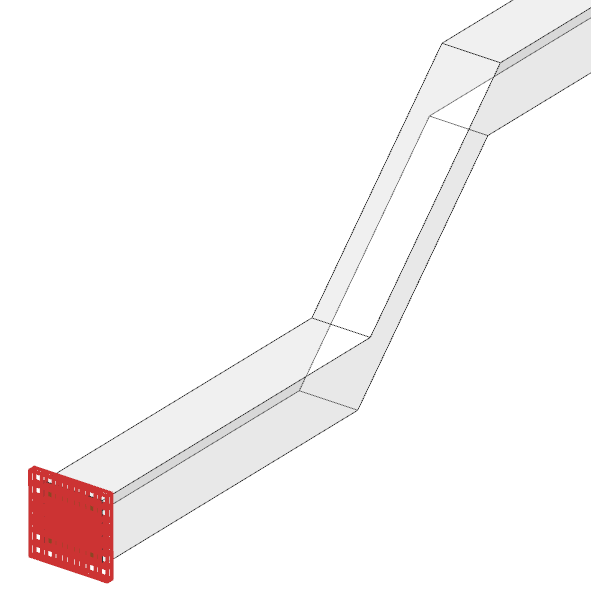
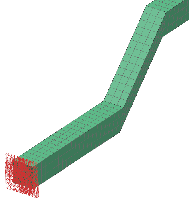
Assign a load ’Current’ of type ’On Solid Face’ to the other
electrode face of the conductor. Assign a value of ’1500 A’.
Create a convection constraint for the coupled thermal solution:
Blank the Air body and choose a constraint of type ’EM Thermal
Constraints’ ![]() .
.
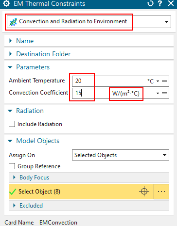
In the dialog set the type to ’Convection and Radiation to
Environment’ ![]() .
.
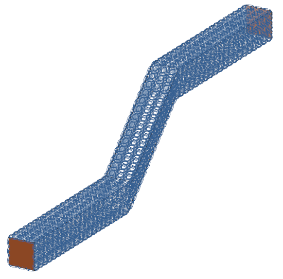
Select the outside faces of the conductor (all faces except the 2
electrode faces. The number of faces is 8). Assign the values for
’Ambient Temperature’ and ’Convection Coefficient’ as shown. Take care
using the shown units.
Solve the solution. The 100 time steps take approximately 2 minutes solve time.
Open the plot results and check them as follows.
Verify that in the ’Initial Time Condition, 0 sec’, there is a temperature of \(20^\circ\)C in the conductor and a current density of zero. This result represents the initial condition and is only of interest for checking.
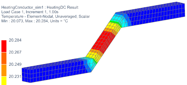
Check the result at time 1 sec.
Temperature is \(20.3^0 C\). Current
density in average is about \(4.6e6
A/m^{2}\).
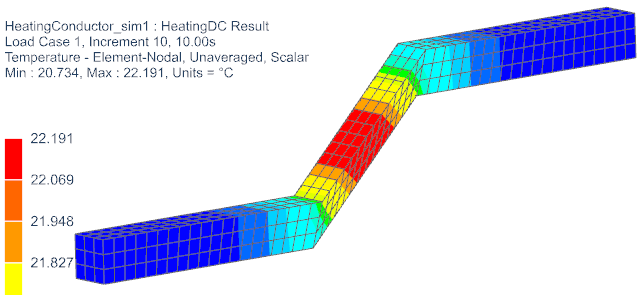
Check the result at time 10 sec.
Temperature in conductor is \(22.2^0
C\).
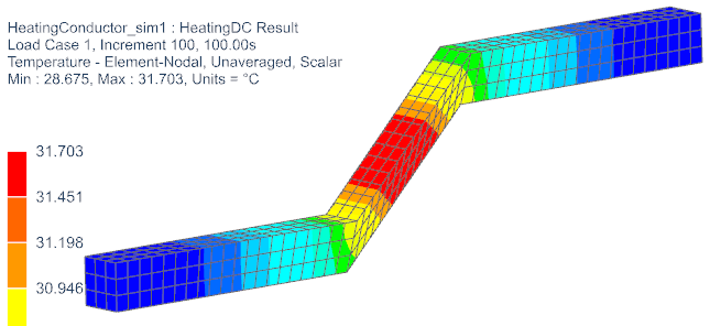
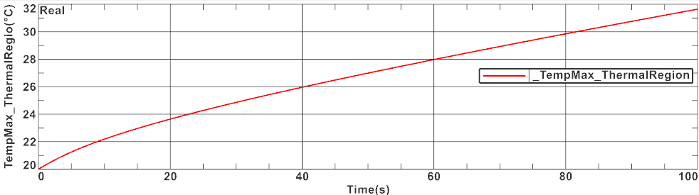
Check the result at time 100 sec.
Temperature is \(31.7^0 C\).
We compare against analytic thermal theory using a basic energy form for heating of conductors. Notice that for simplicity reasons this formula does not include convection effects. \[\begin{aligned} Q &= m \cdot C \cdot \bigtriangleup T \; \Rightarrow \; \bigtriangleup T = \frac{Q}{m \cdot C} \end{aligned}\] with T: Temperature [K], Q: Energy [W s], m: mass[Kg], C: Capacity [W s/K]. Q can easily be determined by the following equations:
\(Q = P \cdot t\)
\(P = R \cdot I^2\)
with P: Power Loss [W], I: Current[A], t: Time[s], R: specific resistance[\(\Omega \cdot \frac{l}{A}\)]. The specific resistance R is defined by the reciprocal value of the conductivity multiplied by the the length of the conductor divided by its cross-section. As the conductor exists of different cross sections, the specific resistance of the different areas can be added up:
\[\begin{aligned}
R=\frac{1}{\sigma} \cdot \sum \frac{l}{A}
\end{aligned}\] The conductivity \(\sigma[S/m]\) can be read from the material
property in NX, the length[m] and cross section[\(m^2\)] of each area can be measured.

By using an excel sheet the resulting delta T values become:
| Delta T [sec] | Temperature Theory [\(^\circ\)C] | Temperature Simulation [\(^\circ\)C] |
|---|---|---|
| 1 | 0.1 | 0.3 |
| 10 | 1 | 2.2 |
| 20 | 2.1 | 3.7 |
| 40 | 4.2 | 6.0 |
| 100 | 10.5 | 11.7 |
which is acceptable close to our simulation results. (subtract 20\(^\circ\)C from the simulation results
because of the initial temperature). At larger time periods the result
differs more and more because of convection effects included in the
simulation.
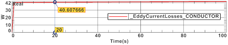
Open the afu file that shows eddy current losses. Check the calculated eddy losses:
Conductor: about 40.6 W.
Using the excel sheet you can check the analytically calculated eddy losses on the conductor. This value is 40.7 W, thus, the simulation losses results are accurate.
Display the graph of temperature maximum over the iterations. The
graph shows that after 100 s there is still no steady state
situation.
To optionally simulate a longer time, period perform these steps:
clone the solution,
Name the new one ’HeatingDCLongTime’.
Change the ’Number of Time Steps’ to 500 and
The ’Time increment’ to 50 sec.
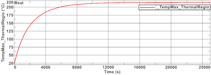
Solve the solution. This will require about 12 minutes time.
Create again the temperature graph over iterations. At the end time the temperature doesn’t change very much any more. Thus, the end temperature (\(214.7^0 C\)) is now near to a steady state situation. We will compare this value in the next example against a simulation that directly solves for steady state.
The eddy current losses have increased to 66.9 W. The reason is that at higher temperatures the electric conductivity decreases and if the current is constant, the losses must increase. We will compare this also against the following steady state solution.
Save your files. In case you want to proceed with the next example, don’t close the files.
This example builds on top of the last one and analyses for the
steady state temperature of the conductor.
Estimated time: 10 min.
Follow the steps to reproduce it:
Open the Sim file ’HeatingConductor_sim1.sim’ generated by the last example. You can either use your own files or those from the ’complete’ folder.
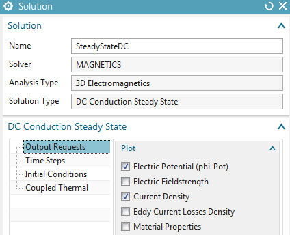
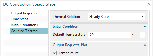
Create a new solution of type ’DC Conduction Steady State’.
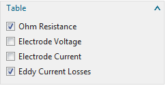
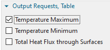
Name this solution ’SteadyStateDC’. Activate the output requests and
thermal solution as shown below.
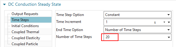
At Time Steps, we should allow some steps because of temperature
dependent material properties: These properties are updated with each
time step and thus the solution becomes more and more accurate. Let’s
use 20 steps and in the result we will see that already 5 steps would be
enough.
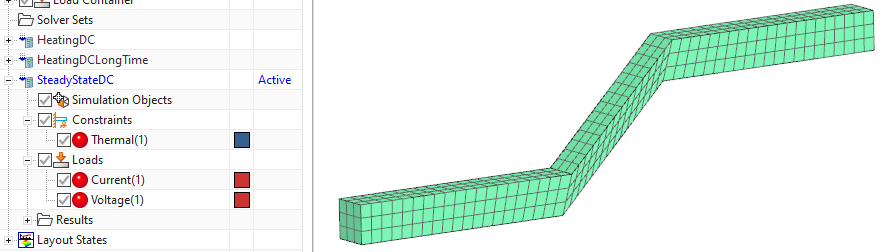
Re-use the ’Thermal’ Constraint with convection. You can do this by ’drag and drop’ the constraint from the container into the constraints of the new solution.
Re-use the ’Current’ and ’Voltage’ loads in the same way.
Solve the solution.
Hint: The air mesh doesn’t play a role in this simulation. Therefore, it
can be deleted, but it can also stay. Another way would be to set it
into a simulation object ’Deactivation Set’.
Open the results and check them:
The Current Density result in the middle of the conductor is about \(7.2 e6 A/m^{2}\). This corresponds to the loaded value of 1500 A on the face area of \(20 mm \cdot 10 mm\).
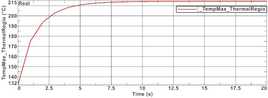
The temperature curve starts at \(132.5^0 C\) and increases up to 214.7 what
is the same value as the long time transient solution gave us. After
about 4 steps there is nearly no change any more. The curve represents
material properties as they update with temperature changes.
Open the corresponding graph file. Check the computed loss value on the conductor after some (4) steps is again 66.5 W as already in the transient solution after long time.
Check the computed ohm resistance. It starts at 1.79e-5 Ohm and finishes with 3.09e-5 Ohm. The start value is near to the analytically value of 1.81e-5 Ohm because the analytic form did not take into account the temperature dependency of material properties.
Save your files. If you want to proceed with the next example don’t close them.
In this example we will apply harmonic current (AC) on the conductor
geometry. In the result we will find eddy current losses on the
conductor. Those losses will lead to heating of the conductor.
Estimated Time: 15 min.
In this first part we will do a magneto-dynamic frequency solution for
the AC magnetic fields with a coupled steady state solution for the
thermal field. This will result in the steady state solution for the
temperature under AC condition.
Follow the steps:
Open the Sim file ’HeatingConductor_sim1.sim’ generated by the last example. You can either use your own files or those from the ’complete’ folder.
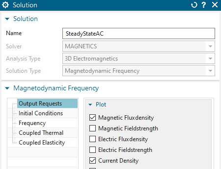
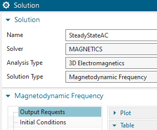
Create a new solution of type ’3D Magnetodynamic
Frequency’.
Name this solution ’SteadyStateAC’. Activate the settings as
shown:
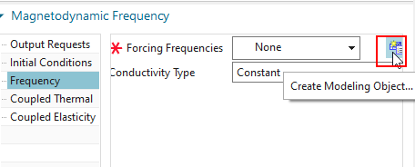
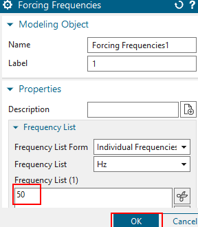
In register ’Frequency’, create a modeling object for the forcing
frequency and accept the default 50 Hz in the list.
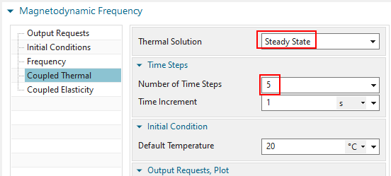
In register ’Coupled Thermal’, set the ’Thermal Solution’ to
’Steady State’. To allow temperature dependent material properties to
converge, we set the number of time steps to 5. The resulting
temperature curve will show the convergence behaviour.
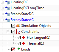
Use both already created constraints ’FluxTangent’, and ’Thermal’
for this solution.
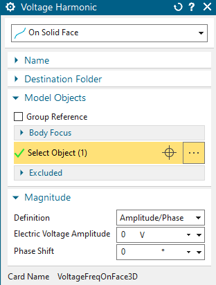
Create a load ’Voltage Harmonic’, set the type to ’On Solid Face’
on one of the electrode faces. Assign 0 V.
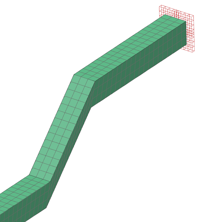
Create a load ’Current Harmonic’ on the other electrode face. Set
the type to ’On Solid Face’. Assign 1500 A.
Solve the solution.
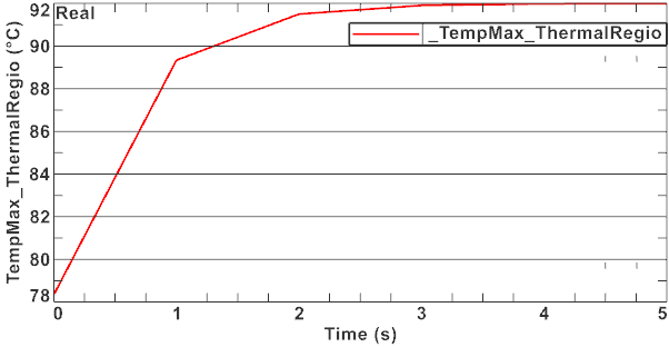
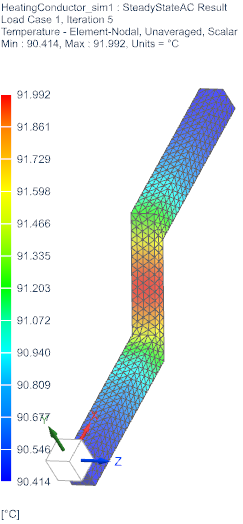
Open the results and display the temperature graph and the plot
results. The converged temperature of about \(91.99^0 C\) resulting from this AC analysis
is lower than the one from DC analysis even if both use 1500 A. The
reason is the lower effective power in AC.
Save your files and close them.
We do the same as in the last example, except the thermal domain will be set to transient. This will result in a step by step heating of the conductor, starting from the initial temperature of \(20^0 C\). When doing this over a long time period, result will be the same as in the steady state case of the last example.
Open the Sim file ’HeatingConductor_sim1.sim’.
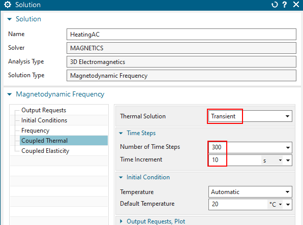
Clone the last created solution ’SteadyStateAC’. Rename the new to ’HeatingAC’.
Edit the solution parameters. In register ’Coupled Thermal’ set
the ’Thermal Solution’ to ’Transient’ and set the settings as shown
below.
Solve the solution.
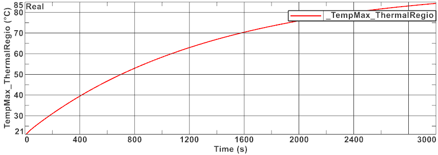
Open the results and show the graph for the conductor maximum
temperature. The temperature at the end of the time period becomes \(84.3^0 C\) and it corresponds adequate to
the one calculated in the previous steady state case (\(91.99^0C\)). Deviation: \(9.1\)%
Save your parts and close them.
At each electrode there is either voltage (U) given and current (I) will result or I is given and then U will result. If the solution runs in frequency domain, such as ’Magnetodynamic Frequency’, then all results are complex, meaning they have an real (Re) and an imaginary (Im) part. For the following explanations we use solution ’SteadyStateAC’.
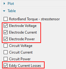
RMB ’Edit’ the solution and activate the following table output
requests: ’Electrode Current’, ’Electrode Voltage’, ’Electrode Power’
and ’Eddy Current Losses’.
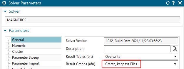
RMB ’Edit Solver Parameters’ for the solution and set the option
’Result Graph Files’ to ’Create, keep txt Files’. This setting allows us
to find the tabular results in simple text files.
Solve the solution.
After solve has finished, check for files with ’txt’ extension in the work directory. There should be one txt file for each requested table result. Such txt files show in one line all results of the electrodes always in this manner: First value is the frequency, second the real value (Re) and third the imaginary value (Im). Using these values many others can be derived, for instance the amplitude is the geometric addition as \(\sqrt{Re^2 + Im^2}\)
Lets start with the current results. Open the file with extension
’.current.txt’ and check the last line (each line is for one time step).
It can be seen that the electrode named ’VoltageHarmonic 1’ has a
current of Re = -1500 A (nearly) and Im = 0 A (nearly). The second
electrode ’CurrentHarmonic 1’ has Re = +1500 A and Im = 0 A. This second
result is not very interesting, because it is what we have assigned, but
the first one is a result from the simulation and it shows great
accuracy.

Now lets check the resulting voltages: Open the file with
extension ’.voltage.txt’. We see that the electrode ’VoltageHarmonic 1’
has a voltage of Re = 0 V and Im = 0 V. This is what we have assigned.
The second one ’CurrentHarmonic 1’ has Re = -0.03059 V and Im = -0.07700
V. This represents the voltage drop over the conductor.

Now check the electrode power results. Open the file with
extension ’.ElectrodePower.txt’. The following results are computed from
the prior U and I by complex multiplication. So we find Re = 0, Im = 0
for ’VoltageHarmonic 1’ and Re = -22.94612 W, Im = -57.75155 W for
’CurrentHarmonic 1’. These give important information: The Re value is
the active or effective power (german Wirkleistung) and the Im value is
the reactive power (german Blindleistung).

In other situations, we may have several electrodes on a conductor, each
showing different values for power. Summing up all the effective powers
(with correct sign) will give the total effective power loss on that
conductor.
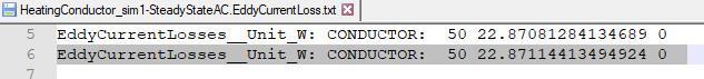
Finally lets check the eddy losses file with extension
’.EddyCurrentLoss.txt’. This file now gives not an electrode but an
integral result over the whole conductor body. It is calculated by the
form \(sigma * SquNorm[-Dt[{a}]-{d
v}]\) what corresponds to the simple form \(R \cdot I^2\). The value computed on the
conductor is 22.87114 W and it well corresponds to the prior effective
power.
The tutorial is complete. Save your files and close them.