These tutorials shall allow the new user to quickly become familiar
with MAGNETICS for Simcenter. Best would be to go through them in the
order listed but it is also possible to start with any of them. The
following three tutorials are especially convenient for beginners:
The Simcenter/NX files for these tutorials can be downloaded as a
zip-archive and the download-link is given at the beginning of each
section. The files of each tutorial have a folder ’complete’ that
contains the files of the completed tutorial. Also a folder called
’start’ exists, that contains the files to start with when going through
the exercise.
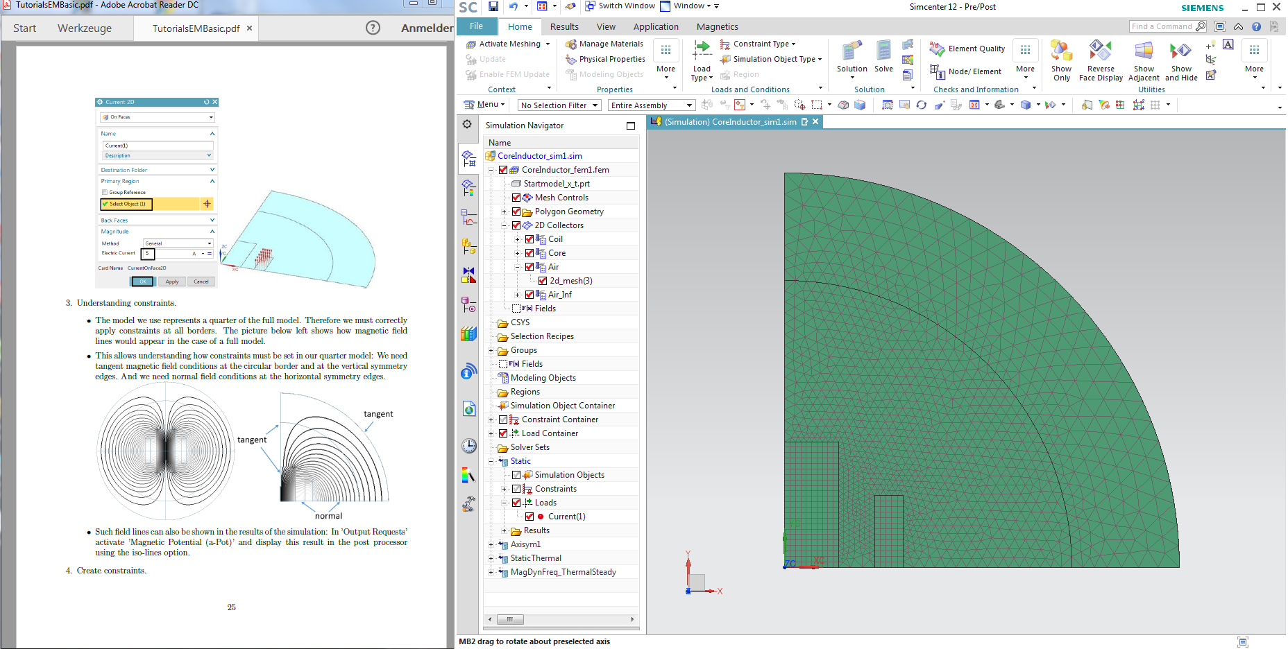
We recommend, when working through the tutorials, positioning this pdf
and the Simcenter window side by side on your screen (see picture
below).
Now we wish all users a lot of success in learning and performing
electromagnetic simulations with MAGNETICS for Simcenter 3D or NX.
In case of problems please write to the support address
cae-support@drbinde.de and our team will be there for you.
With best wishes, your team of Dr. Binde Ingenieure
Electromagnetic
Principles
This section is based on the lecture notes on ’Applied &
Computational Electromagnetics’ from the University of Liège [Geuzaine
2013], on [Binde] and on [Kost].
In the context of electromagnetic fields, Maxwell’s equations are
solved. Depending on the application, e.g. electrostatic or
magnetodynamics, the equations are simplified or only subsets are
considered. For the solution of the equations, the finite element method
has been established.
In the following, we provide the usual governing electromagnetic
equations, Maxwell’s equations and material relations that are the
foundations of said models. We then explain which type of model is the
right one for a certain application problem, and finally provide the
equations that belong to the individual models.
Maxwell Equations
Let’s look at the Maxwell equations that describe the electromagnetic
effects and are the basis for the models or applications listed above.
Maxwell’s equations are a set of four equations.
Magnetic fluxdensity \(\mathbf{B}\) has no sources.
Instead of the capital letters for the vector fields \(\mathbf{H}, \mathbf{B}, \mathbf{E}, \mathbf{D},
\mathbf{J}\) we will also use small letters
h,b,e,d,j for them, especially when writing
the formulations into the solver input file.
Material Equations
In order to properly specify the system (i.e. we have 16 unknowns
from the fields and sources but only 7 equations when considering the
continuity equation), additional equations are needed: the material
equations. By applying material laws magnetic and electrical material
properties are included in the analysis. There exist three material
laws.
Equation name
Form
Remarks and units
Magnetic relationship
\(\mathbf{B} =
\mu \cdot \mathbf{H}\)
Magnetic permeability \(\mu\) is the basic property.
\(\mu\)
is often nonlinear. Then, a \(BH\)
curve is given.
Usually \(\mu =
\mu_{0} \cdot \mu_{r}\) is used.
Dielectric relationship
\(\mathbf{D} =
\epsilon \cdot \mathbf{E}\)
Electric permittivity \(\epsilon\) is the basic property.
Ohm’s law
\(\mathbf{J} =
\sigma \cdot \mathbf{E}\)
Electric conductivity \(\sigma \space [S/m]\) is basic
property.
Electromagnetic
Models
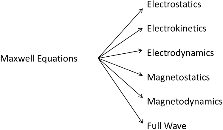
The below picture shows use cases of interest in the electromagnetic
analysis area which can arise from the Maxwell equations.
The six principle submodels that can be derived from the Maxwell
equations particularly differ in the way they account for the effects
capacitance, ohm resistance and inductivity. Accordingly, icons for
capacitor, resistor and coil can be assigned:
Electrostatics: here static charges or electrical voltages are the key
ingredient and are thus set as sources. As a result of the simulation,
we obtain the electric field distribution. This corresponds to a
consideration of the capacitive properties (hence the symbol of a
capacitor).
Electrokinetic (DC Conduction): here, we consider the static distribution of electricity
in conductors. The most important feature is the electrical conductivity
or the ohm resistance (hence the symbol of resistance).
Electrodynamics: This is a combination of electrostatics and kinetics.
The distribution of the electric field and electric currents in
materials (conductors and insulators) are considered. It can also lead
to dynamic effects.
Magnetostatics: We consider the static magnetic field, which can result
from permanent magnets and stationary electric currents. As this
corresponds to the effect of the inductance, we select the icon of the
coil. Read more about this in chapter ’Magnetostatics’.
Magnetodynamics: Result is the magnetic field and eddy currents (Eddy
Currents), which result from moving magnets or time-varying currents. A
suitable symbol is the coil with ohm resistance, because these two
effects are considered.
Full Wave (High Frequency): This includes considering the full electromagnetic
waves. It requires that all three effects of capacitance, resistance and
inductance are taken into account. This allows to determine vibrations
and resonances, therefore the symbol of the electrical resonant circuit
is suitable.
 : here static charges or electrical voltages are the key
ingredient and are thus set as sources. As a result of the simulation,
we obtain the electric field distribution. This corresponds to a
consideration of the capacitive properties (hence the symbol of a
capacitor).
: here static charges or electrical voltages are the key
ingredient and are thus set as sources. As a result of the simulation,
we obtain the electric field distribution. This corresponds to a
consideration of the capacitive properties (hence the symbol of a
capacitor). : here, we consider the static distribution of electricity
in conductors. The most important feature is the electrical conductivity
or the ohm resistance (hence the symbol of resistance).
: here, we consider the static distribution of electricity
in conductors. The most important feature is the electrical conductivity
or the ohm resistance (hence the symbol of resistance). : This is a combination of electrostatics and kinetics.
The distribution of the electric field and electric currents in
materials (conductors and insulators) are considered. It can also lead
to dynamic effects.
: This is a combination of electrostatics and kinetics.
The distribution of the electric field and electric currents in
materials (conductors and insulators) are considered. It can also lead
to dynamic effects. : We consider the static magnetic field, which can result
from permanent magnets and stationary electric currents. As this
corresponds to the effect of the inductance, we select the icon of the
coil. Read more about this in chapter ’Magnetostatics’.
: We consider the static magnetic field, which can result
from permanent magnets and stationary electric currents. As this
corresponds to the effect of the inductance, we select the icon of the
coil. Read more about this in chapter ’Magnetostatics’. : Result is the magnetic field and eddy currents (Eddy
Currents), which result from moving magnets or time-varying currents. A
suitable symbol is the coil with ohm resistance, because these two
effects are considered.
: Result is the magnetic field and eddy currents (Eddy
Currents), which result from moving magnets or time-varying currents. A
suitable symbol is the coil with ohm resistance, because these two
effects are considered. : This includes considering the full electromagnetic
waves. It requires that all three effects of capacitance, resistance and
inductance are taken into account. This allows to determine vibrations
and resonances, therefore the symbol of the electrical resonant circuit
is suitable.
: This includes considering the full electromagnetic
waves. It requires that all three effects of capacitance, resistance and
inductance are taken into account. This allows to determine vibrations
and resonances, therefore the symbol of the electrical resonant circuit
is suitable.