Acoustics of Transformer with Housing

In this example we want to analyse for the acoustics that result from magnetic forces on a transformer. There are three main steps to do:

First, in a time domain analysis we compute the magnetic forces that act on the transformer and its housing. In the second step, we transfer those forces into frequency domain by using a solution type that provides fourier transformation (FFT). In the last step we perform a Simcenter Nastran, vibro-acoustic simulation with the forces from magnetics.

Estimated time: 1.5 h.

Follow the steps:

Create Model for Magnetic Forces

1. download and unzip the model files for this tutorial from the following link:
   https://www.magnetics.de/downloads/Tutorials/15.CouplAcoustics/15.1TrafoHousing.zip

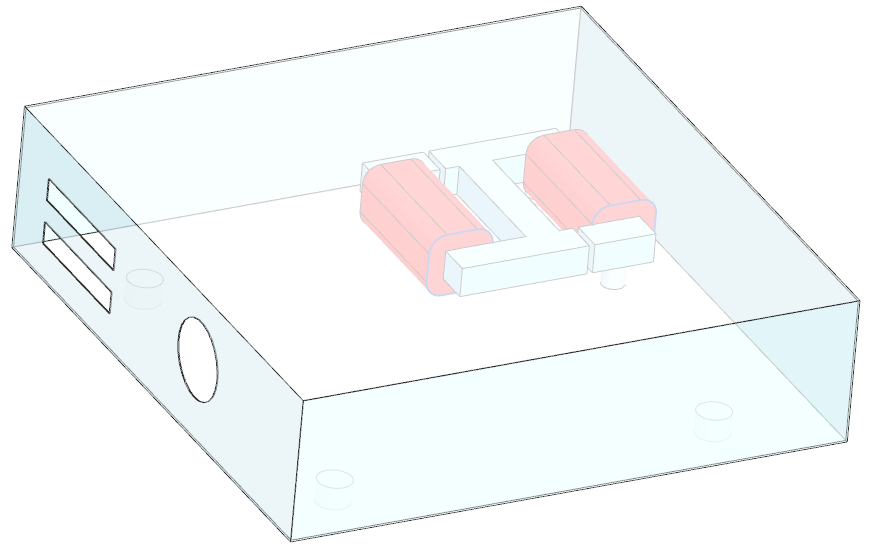
2. Start Simcenter, click Open and navigate to folder ’start’. Select the file ’TrafoHousingAcoustic.prt’ and click OK.

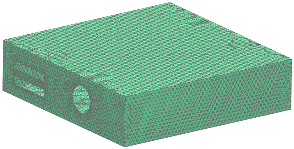
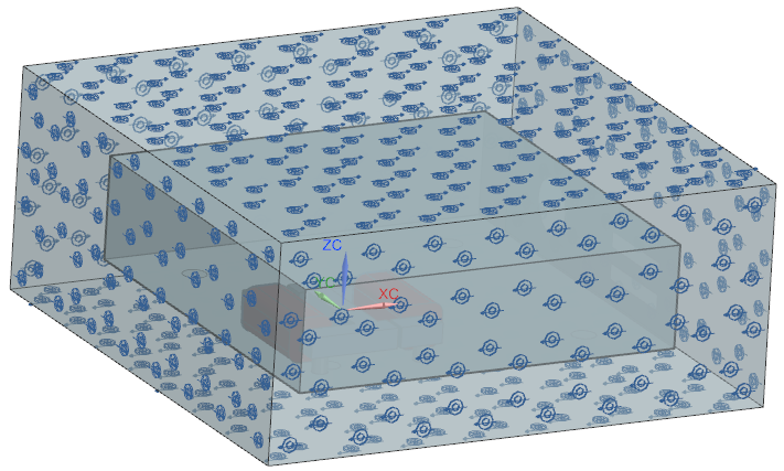
3. Check the bodies and the air volume around the housing.

4. Start application Pre/Post and click ’New Fem and Sim (Non-Manifold)’ from toolbar Magnetics .

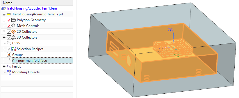
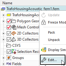
5. Change the displayed part to the Fem part.

6. Check the non-manifold faces: In ’Groups’, check that there is a group named ’non-manifold face’. Select the group and verify that the correct faces highlight. Such faces show the interfaces (matings) between two bodies. Here, the mesh must be conformal (identical nodes).
   

7. Blank the AIR_EMAG and the HOUSING polygon bodies for easier visibility and selection.

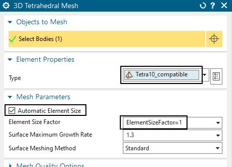
8. Use the tetrahedral mesher with following settings.

   • Set the ’Type’ to ’Tetra10_compatible’.
     Hint: For the Magnetics solver, this makes no difference. But this setting allows to use this mesh as a Tetra10 mesh if the Nastran solver runs. Thus, we can use these meshes for both solvers now.

   • with activated ’Automatic Element Size’ and

   • ’ElementSizeFactor’ = 1 to mesh the bodies in the following order (small parts first).
     Hint: We use a coarse mesh to speed up the process. Later, to find precise results, the ’ElementSizeFactor’ can be set to 0.5 or 0.25.
     

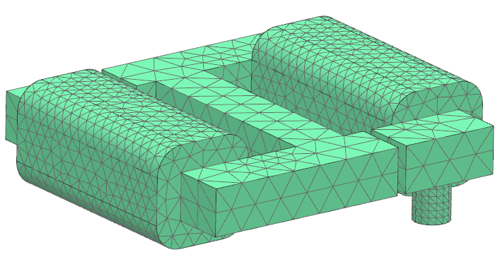
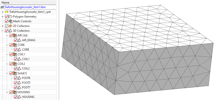
9. Mesh the bodies and set the materials as shown in brackets.

   • CORE (Material: ’MU3: Relative permeability 1000’)

   • COIL1, COIL2 (Material: ’Copper: 5.77e7 Siemens/meter’)

   • FOOT1, ..., FOOT7 (Material: ’Aluminum: 3.8e7 Siemens/meter’)

   • HOUSING (Material: Material: ’Aluminum: 3.8e7 Siemens/meter’)
     

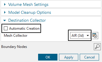
10. Finally, unblank the AIR_EMAG polygon body and mesh it in the same way.

    • Put this mesh into the existing mesh collector ’AIR (3d)’.
      

    • blank all meshes for easier visibility.

11. Define the coils:

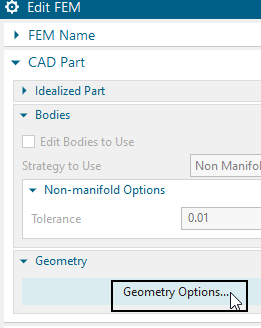
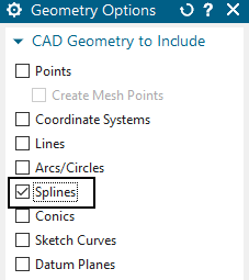
    • Edit the Fem file and in ’Geometry Options’, activate ’Splines’.
      

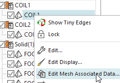
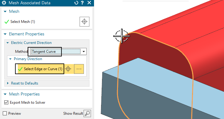
    • Edit the ’Mesh Associated Data’ of both coil meshes, set the ’Method’ to ’Tangent Curve’ and for each coil, select the spline as shown in below picture.
      

    • Edit Physical property of COIL1 and COIL2.

      • Set the ’Conductor Type’ to ’Stranded’,

      • the ’Coil Section Area’ to 120*15 mm

      • the ’Number of Turns’ to 90

      • the ’Fill Factor’ to 0.8

12. Set the displayed part to the Sim file.

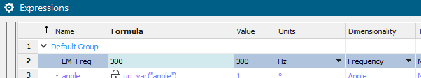
13. create a expression (shortcut Strg+E) for the main frequency that we want to use. Name it ’EM_Freq’, set the ’Dimensionality’ to ’Frequency’ and use 300 Hz as formula.
    

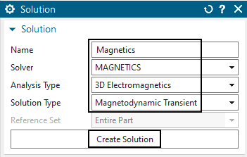
14. Create a new Solution for the Magnetics solver. Solution Type is ’Magnetodynamic Transient’

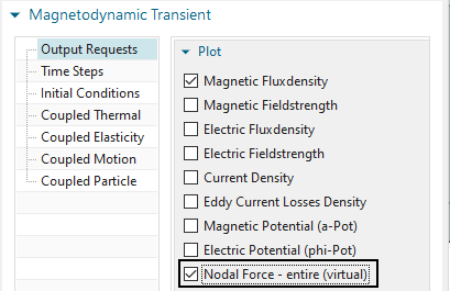
15. in register ’Output Requests’, ’Plot’, activate ’Nodal Force - entire (virtual)’.
    Hint: This is the necessary output for the following fourier-transformation and acoustic simulation. Other results can be activated also if desired.
    

16. in register ’Table’, activate ’Total Force - entire (virtual)’ to allow post processing of these.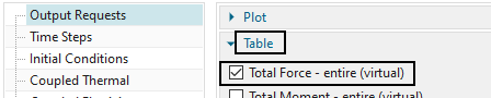

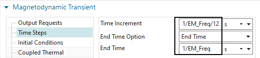
17. in register ’Time Steps’,

    • set the ’End Time Option’ to ’End Time’

    • and the ’End Time’ to ’1/EM_Freq’.

    • set the ’Time Increment’ to ’1/EM_Freq/12’.
      Thus, we will have 12 time steps going over one period depending on the defined frequency. Hint: This is a coarse time step. For higher accuracy, make it smaller.
      

18. Click Ok to finish the solution window.

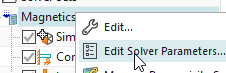
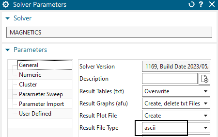
19. Edit the ’Solver Parameter’. In register ’General’, set the ’Result File Type’ to ’ascii’.
    Hint: the result will be written in readable ascii format now. This is necessary for the following fourier-transformation. As a disadvantage, the reading and writing of results will be slower as in the default binary setting.
    

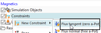
20. Create a constraint of type ’Flux Tangent’ on all 6 outside faces of the air volume.
    

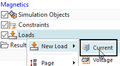
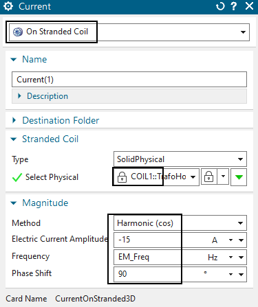
21. On each coil, create a load of type ’Current’.

    • Use the default type ’On Stranded Coil’

    • Select the Physical: COIL1 and COIL2 for the second.

    • Set the ’Method’ to ’Harmonic (cos)’,

    • ’Electric Current Amplitude’ to -15 A

    • ’Frequency’ to ’EM_Freq’

    • ’Phase Shift’ to 90 deg.
      
      

22. Save the Sim file

23. Solve the Magnetics solution. The solve time will be approximately 5 min.

24. Postprocess the results if desired.

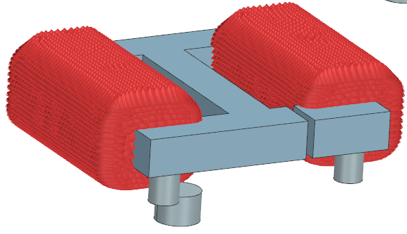
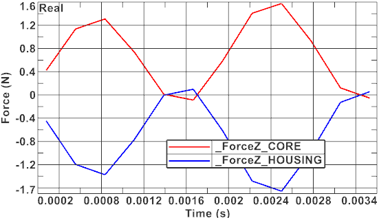
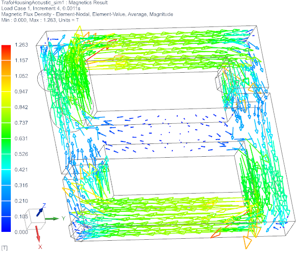
25. The following picture left shows the total forces in z on the core and on the housing. The right picture shows the Magnetic Fluxdensity in the core (Post View set to Combine at Elements).
    

Fourier-Transform Magnetic Forces

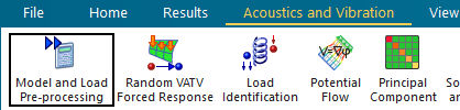
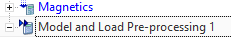
1. from toolbar ’Acoustics and Vibration’ (maybe this toolbar is invisible, thus, make it visible first), Click on ’Model and Load Pre-processing’. A new solution will be created and visible in the Simulation-Navigator.
   

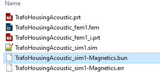
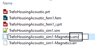
2. Use the Windows file manager to rename the Magnetics results file-extension from ’bun’ to ’unv’.
   Hint: Our magnetics result file is now formatted with ascii type (we have requested that above). Normally, such files are then named with ’unv’ extension (universal file) but our file has still the extension ’bun’ (binary universal file). Thus, we must rename it for further usage. Maybe you must unload it in the postprocessor to allow Windows to rename it. Making a copy of the file also works.
   

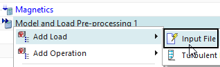
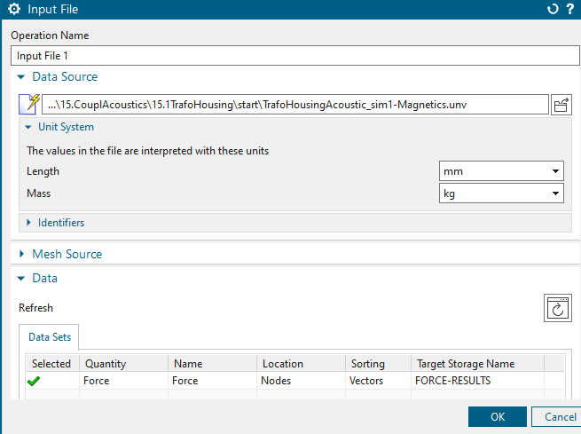
3. In the solution ’Model and Load Processing’, ’Add a Load’ for the ’Input File’.

4. in the file browser, select the Magnetics results file (extension ’unv’)

5. in box ’Unit System’, set ’Length’ to mm.

6. click the ’Refresh’ button and verify that the data set ’Force’ is found.

7. click OK.
   

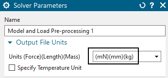
8. There is another unit setting that must also be changed: Edit the solution ’Model and Load Processing’ and set the ’Output File Units’ to (mN)(mm)(Kg)
   

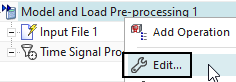
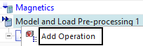
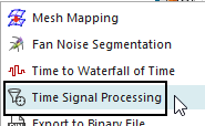
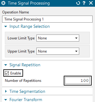
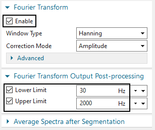
9. In the solution ’Model and Load Processing’, click ’Add Operation’ and select ’Time Signal Processing’.
   

10. Set the properties as shown in the below picture. Click OK.
    

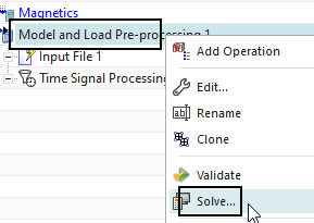
11. Solve the solution ’Model and Load Processing’. The solve time is about 3 min.
    

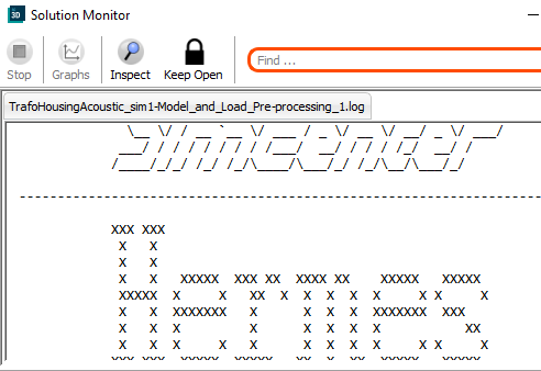
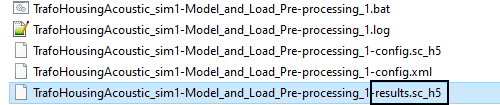
12. after the solve has finished, verify in the Windows file manager that there is a new file generated with extension ’results.sc_h5’.
    

Create Model for Acoustics

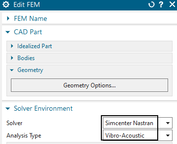
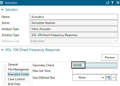
1. In the Sim file, create a new solution,

   • Name it ’Acoustics’

   • set the solver to Simcenter Nastran

   • set the ’Analysis Type’ to ’Vibro-Acoustic’

   • set the ’Solution Type’ to ’SOL 108 Direct Frequency Response’
     Hint: Other solution types are also possible.
     

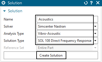
   • click ’Create Solution’

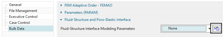
   • in register ’Bulk Data’, in box ’Fluid-Structure and Poro-Elastic Interface’, create a Modeling-object for ’Fluid-Structure Interface Modeling Parameters’
     

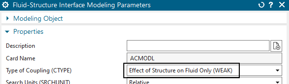
   • set the ’Type of Coupling’ to ’Effect of Structure on Fluid Only (WEAK)’
     

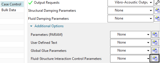
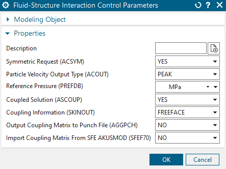
   • in register ’Case Control’, in box ’Additional Options’, create a Modeling-object for ’Fluid-Structure Interaction Control Parameters’ and accept all the defaults.
     

   • Click OK to create the solution.
     

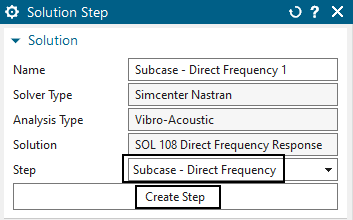
   • A new window ’Solution Step’ appears. Accept the default step ’Direct Frequency’. click ’Create Step’ and OK.

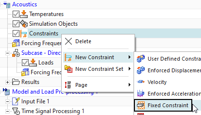
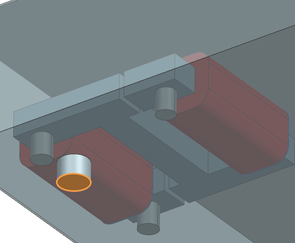
2. Create a constraint of type ’Fixed’ on one of the foot faces.
   

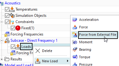
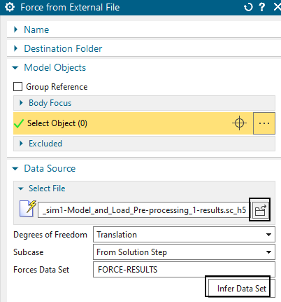
3. Create a load of type ’Force from External File’

   • use the file browser and select the newly created file with extension ’results.sc_h5’

   • click the button ’Infer Data Set’

   • click OK and the load is generated.

   

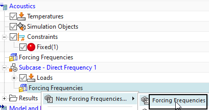
4. Create Forcing Frequencies
   

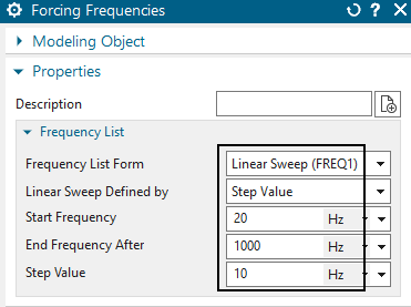
5. Prepare the Fem part for acoustics

   • Change the displayed part to the Fem file

   • Edit the Fem part and set the solver to Simcenter Nastran and the ’Analysis Type’ to ’Vibro-Acoustics’
     

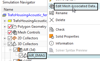
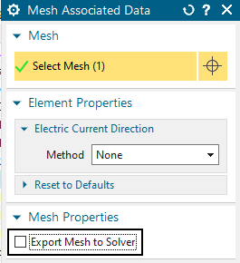
   • Deactivate the air-mesh that was used for electromagnetics: Edit the ’Mesh Associated Data’ and deactivate the option ’Export to Solver’
     

   • blank all meshes, blank also the AIR_EMAG polygon body. Unblank all other polygon bodies.

6. Create the acoustics mesh

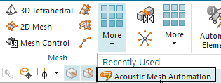
   • from toolbar ’Home’, group ’Mesh’, select ’Acoustic Mesh Automation’
     

   • drag a window to select all polygon bodies (not the AIR_EMAG)

   • set the ’Element Size’ to 10 mm at both ’Acoustic Shell Surface Wrap’ and ’Convex Mesh’

   • set the ’Offset Distance’ to 50 mm.
     

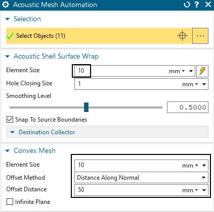
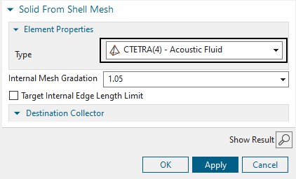
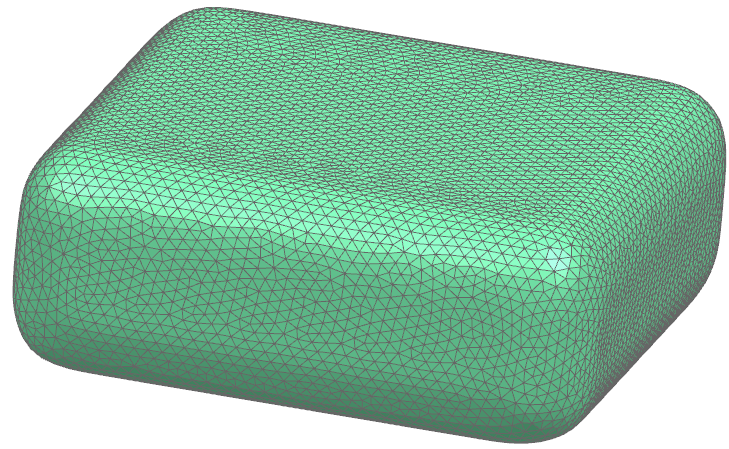
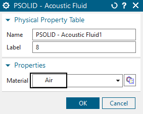
   • click OK and the mesh is created. Assign material Air to it.
     

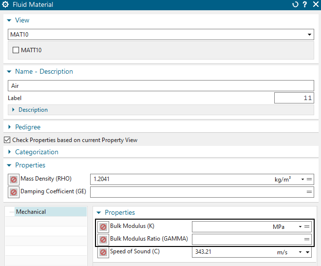
   • edit the Material ‘Air‘ and disable ’Bulk Modulus’ and ’Bulk Modulus Ratio’.
     
     

   • blank the acoustic air mesh and also the 2D meshes that have been created.

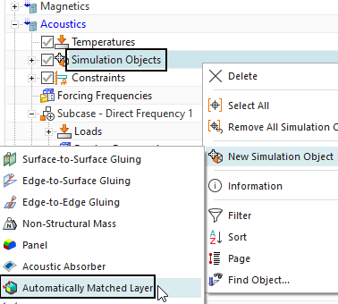
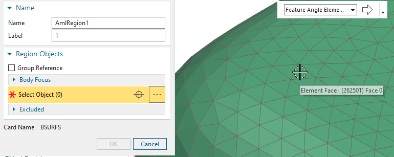
7. Create an Automatically Matched Layer (AML)

   • Create a Simulation Object of type ’Automatically Matched Layer’.
     

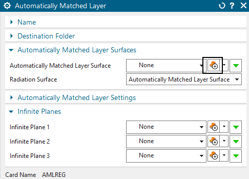
   • click ’Create Region’ and set the selection filter to ’Feature Angle Element Face’ and select one of the outside element faces of the acoustic air mesh. All others will be selected. Click OK twice to create the condition.
     

8. Create microphone meshes

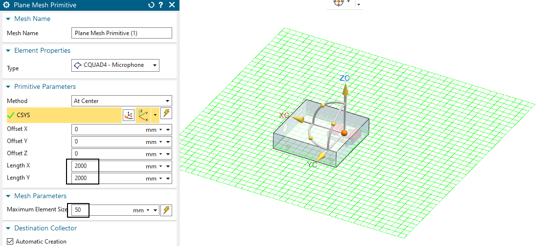
   • from toolbar ’Nodes and Elements’, group ’Elements’, create a ’Plane’
     

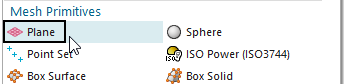
   • set the parameters as shown in the picture for the first plane and click OK.
     

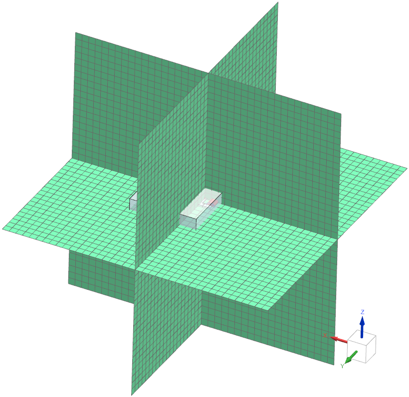
   • do the same for the two other orientations.
     

9. change the displayed part to the Sim file.

10. There are some errors in the mesh, which would not allow us to solve the solution. Therefor we can either fix those errors by using smaller element sizes or we can disable the mesh check from the solution. We are going to use the second option, since decreasing the element sizes exponentially increases the time it takes to solve.

    To disable the error check, edit the solution and change the ‘Geometry Check‘ in ‘Executive Control‘ to ‘None‘.
    
    

11. solve the acoustic solution. The needed time is about 1.5h.

Postprocess Acoustic Results

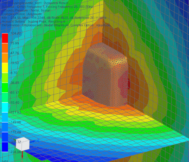
1. In the post-processor, open the result from the acoustic simulation

2. choose the frequency 300 Hz and show the result ’Acoustic Pressure’

3. Edit the Postview and in ’Result’, activate ’Apply dB Scaling’

4. Measuring the sound pressure spectrum at one point

   • Click on ’Create Graph’

   • set it to ’Across Iterations’

   • select one node at a location where we want to measure the sound pressure. Choose for instance a location with a high pressure.

   • click OK. The graph will be created. We can see that there are peaks at the main frequency 300 Hz and multiplications of it 600, 900 Hz. Values below 0 dB mean the sound is below the reference and not possible to hear.
     

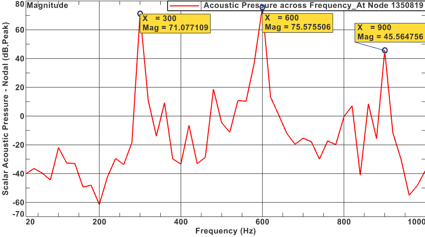
   • the below picture shows the plot of the acoustic pressure.
     

The tutorial is finished. Save your parts and close them.

References:

• Simcenter Nastran Acoustics User’s Guide

• Simcenter Nastran Quick Reference Guide